Query Performance Data

The benchpark query command searches one or more directories for Caliper .cali files and writes selected metadata or performance data to a CSV file. It is useful when you want tabular data for custom plotting or downstream analysis instead of the pre-defined figures generated by benchpark analyze.

benchpark query requires Caliper data generated by an experiment using the Caliper modifier, such as caliper=time,mpi (Benchpark Modifiers). It uses the Thicket performance analysis library to read the Caliper files.

benchpark query requires the same additional Python packages as benchpark analyze. Install them by running pip install .[analyze] in the Benchpark directory.

To query a metadata metric:

$ benchpark query wkp/kripke/cuda/strong/lassen/workspace/ --metric Final-FOM

To query a performance metric for matching regions:

$ benchpark query wkp/kripke/cuda/strong/lassen/workspace/ \
    --metric "Avg time/rank" \
    --query-regions-byname main

For example, this command queries the Problem region from a Frontier ROCm workspace and excludes MPI regions:

$ benchpark query wkp/rocm642-frontier/amg2023/ --query-regions-byname Problem --metric "Avg time/rank" --exclude-regions MPI_
query-20260811-181919.csv

The generated CSV contains one row per matching Caliper profile. Duplicate values in the metadata columns can occur when the workspace contains multiple trials for the same experiment configuration. Lines beginning with # are comments. The first comment records the command line. The trailing comments record the queried call tree structure after region selection and exclusion:

# benchpark query wkp/rocm642-frontier/amg2023/ --query-regions-byname Problem --metric 'Avg time/rank' --exclude-regions MPI_
cluster,application_name,Avg time/rank
frontier,amg2023,7.8742357827500005
frontier,amg2023,7.9076165642800005
frontier,amg2023,7.98603465824
frontier,amg2023,8.17716916271
frontier,amg2023,7.905229214139999

# Problem
# ├─ Setup
# │  ├─ hipDeviceSynchronize
# │  ├─ hipGetDevice
# │  ├─ hipGetDevicePropertiesR0600
# │  ├─ hipGetLastError
# │  ├─ hipHostMalloc
# │  ├─ hipLaunchKernel
# │  ├─ hipMalloc
# │  ├─ hipMemcpy
# │  ├─ hipMemcpyAsync
# │  ├─ hipMemcpyWithStream
# │  ├─ hipMemset
# │  ├─ hipMemsetAsync
# │  ├─ hipPeekAtLastError
# │  └─ hipStreamSynchronize
# └─ Solve
#    ├─ hipDeviceSynchronize
#    ├─ hipGetDevice
#    ├─ hipGetDevicePropertiesR0600
#    ├─ hipGetLastError
#    ├─ hipLaunchKernel
#    ├─ hipMemcpy
#    ├─ hipMemcpyWithStream
#    ├─ hipMemsetAsync
#    ├─ hipPeekAtLastError
#    └─ hipStreamSynchronize

The command writes a file named query-YYYYMMDD-HHMMSS.csv in the current working directory and prints the filename.

Region Queries

When --metric names a performance data column instead of a metadata column, provide at least one region selector:

• --query-regions-byname selects regions and their children whose name contains one of the provided strings.

• --filter-regions-byname keeps regions whose name matches one of the provided prefixes.

• --exclude-regions removes regions and their children whose name contains one of the provided strings before the query is evaluated.

For example, to query computation regions while excluding MPI regions:

$ benchpark query wkp/kripke/cuda/strong/lassen/workspace/ \
    --metric "Avg time/rank" \
    --query-regions-byname Solve Generate \
    --exclude-regions MPI_

Metadata Columns

The CSV always includes cluster and application_name. Use --metadata-columns to include additional metadata columns in the output:

$ benchpark query wkp/kripke/cuda/strong/lassen/workspace/ \
    --metric "Avg time/rank" \
    --query-regions-byname main \
    --metadata-columns n_nodes processes_per_node

The command accepts these arguments:

benchpark query arguments

Argument	Description
DIRECTORY [DIRECTORY ...]	One or more directories to recursively search for Caliper .cali files.
--metric METRIC	Metadata or performance metric to write to the CSV.
--query-regions-byname REGION [REGION ...]	Region name substrings to query.
--filter-regions-byname PREFIX [PREFIX ...]	Region path prefixes to keep.
--metadata-columns COLUMN [COLUMN ...]	Additional metadata columns to include in the CSV.
--exclude-regions PATTERN [PATTERN ...]	Region name substrings to exclude before evaluating the query.

Stacked Bar Chart Example

The following workflow uses benchpark query to split Caliper timing into computation and communication CSV files, then plots the results as stacked bar charts. This example compares ROCm versions using the packages.dependencies.hip.version metadata column.

First, query the computation regions. The notebook version loops over the available wkp/<rocm-version>-<system>/<application>/ directories and appends each generated query CSV into computation-time.csv.

$ benchpark query \
    wkp/rocm720-tioga/amg2023/ wkp/rocm642-tioga/amg2023/ \
    wkp/rocm720-tuo/amg2023/ wkp/rocm642-tuo/amg2023/ \
    --query-regions-byname Problem \
    --metric "Avg time/rank (exc)" \
    --metadata-columns packages.dependencies.hip.version \
    --exclude-regions MPI_

$ benchpark query \
    wkp/rocm720-tioga/kripke/ wkp/rocm642-tioga/kripke/ \
    wkp/rocm720-tuo/kripke/ wkp/rocm642-tuo/kripke/ \
    --query-regions-byname Solve \
    --metric "Avg time/rank (exc)" \
    --metadata-columns packages.dependencies.hip.version \
    --exclude-regions MPI_

$ benchpark query \
    wkp/rocm720-tioga/laghos/ wkp/rocm642-tioga/laghos/ \
    wkp/rocm720-tuo/laghos/ wkp/rocm642-tuo/laghos/ \
    --query-regions-byname SolveVelocity-ForcePA SolveEnergy-ForcePA \
        SolveVelocity-CGVMass QUpdate-UpdateQuadratureData \
    --metric "Avg time/rank (exc)" \
    --metadata-columns packages.dependencies.hip.version \
    --exclude-regions MPI_ SolveEnergy-CGEMass

Then query communication regions by selecting the same parent regions and filtering to MPI_ children. These generated CSV files are appended into communication-time.csv.

$ benchpark query \
    wkp/rocm720-tioga/amg2023/ wkp/rocm642-tioga/amg2023/ \
    wkp/rocm720-tuo/amg2023/ wkp/rocm642-tuo/amg2023/ \
    --query-regions-byname Problem \
    --filter-regions-byname MPI_ \
    --metric "Avg time/rank (exc)" \
    --metadata-columns packages.dependencies.hip.version

$ benchpark query \
    wkp/rocm720-tioga/kripke/ wkp/rocm642-tioga/kripke/ \
    wkp/rocm720-tuo/kripke/ wkp/rocm642-tuo/kripke/ \
    --query-regions-byname Solve \
    --filter-regions-byname MPI_ \
    --metric "Avg time/rank (exc)" \
    --metadata-columns packages.dependencies.hip.version

$ benchpark query \
    wkp/rocm720-tioga/laghos/ wkp/rocm642-tioga/laghos/ \
    wkp/rocm720-tuo/laghos/ wkp/rocm642-tuo/laghos/ \
    --query-regions-byname SolveVelocity-ForcePA SolveEnergy-ForcePA \
        SolveVelocity-CGVMass QUpdate-UpdateQuadratureData \
    --filter-regions-byname MPI_ \
    --metric "Avg time/rank (exc)" \
    --metadata-columns packages.dependencies.hip.version

For applications that do not provide comparable Caliper regions, the same CSV shape can be produced from application output. The notebook parses LAMMPS timing rows into the same cluster, application_name, packages.dependencies.hip.version, and Avg time/rank (exc) columns before appending them to the two CSV files.

The plotting notebook reads both query outputs and groups by system, benchmark, ROCm version, and region type:

import pandas as pd

df_comp = pd.read_csv("computation-time.csv")
df_comm = pd.read_csv("communication-time.csv")

value_col = "Avg time/rank (exc)"
version_col = "packages.dependencies.hip.version"
group_cols = ["cluster", "application_name", version_col]

bar_df = (
    pd.concat(
        [
            df_comp.assign(region="Computation"),
            df_comm.assign(region="Communication"),
        ],
        ignore_index=True,
    )
    .groupby(group_cols + ["region"])[value_col]
    .mean()
    .unstack(fill_value=0)
    .reset_index()
)
bar_df["total"] = bar_df["Computation"] + bar_df["Communication"]

For example, the following code creates a simple stacked bar chart for AMG2023. Each bar represents one system and ROCm version:

import matplotlib.pyplot as plt

amg_df = bar_df[bar_df["application_name"] == "amg2023"].set_index(
    ["cluster", version_col]
)

ax = amg_df[["Computation", "Communication"]].plot.bar(stacked=True)
ax.set_xlabel("System and ROCm version")
ax.set_ylabel("Average time per rank (seconds)")
plt.tight_layout()
plt.show()

The generated figures show computation and communication time stacked together for each benchmark/system pair, with hatching used to distinguish ROCm versions.

Note

The following figures contain extra styling that is not provided in the simplified code snippet above.

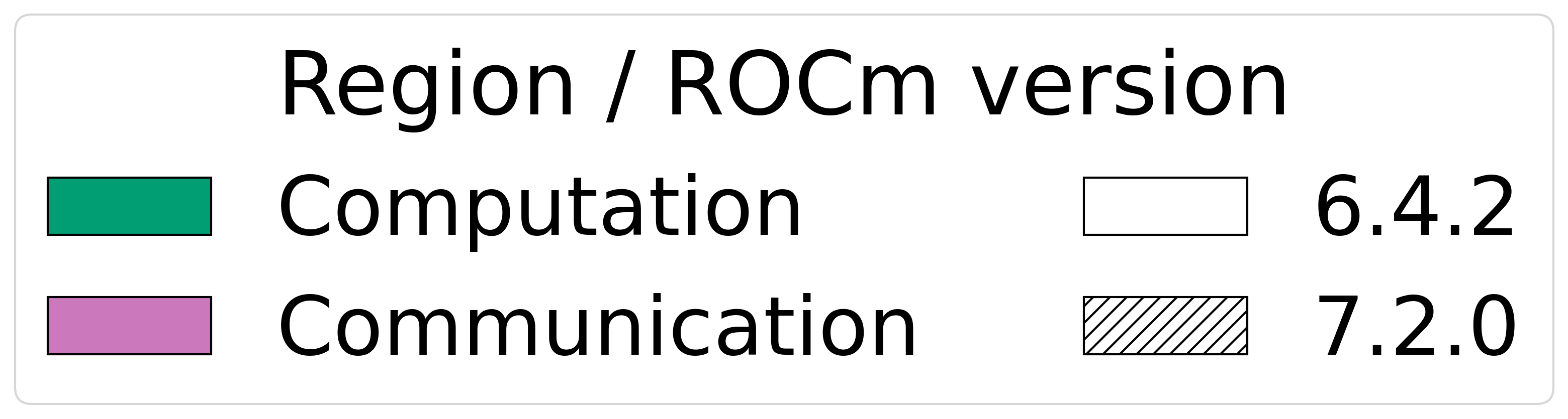
Legend for the stacked bar charts.

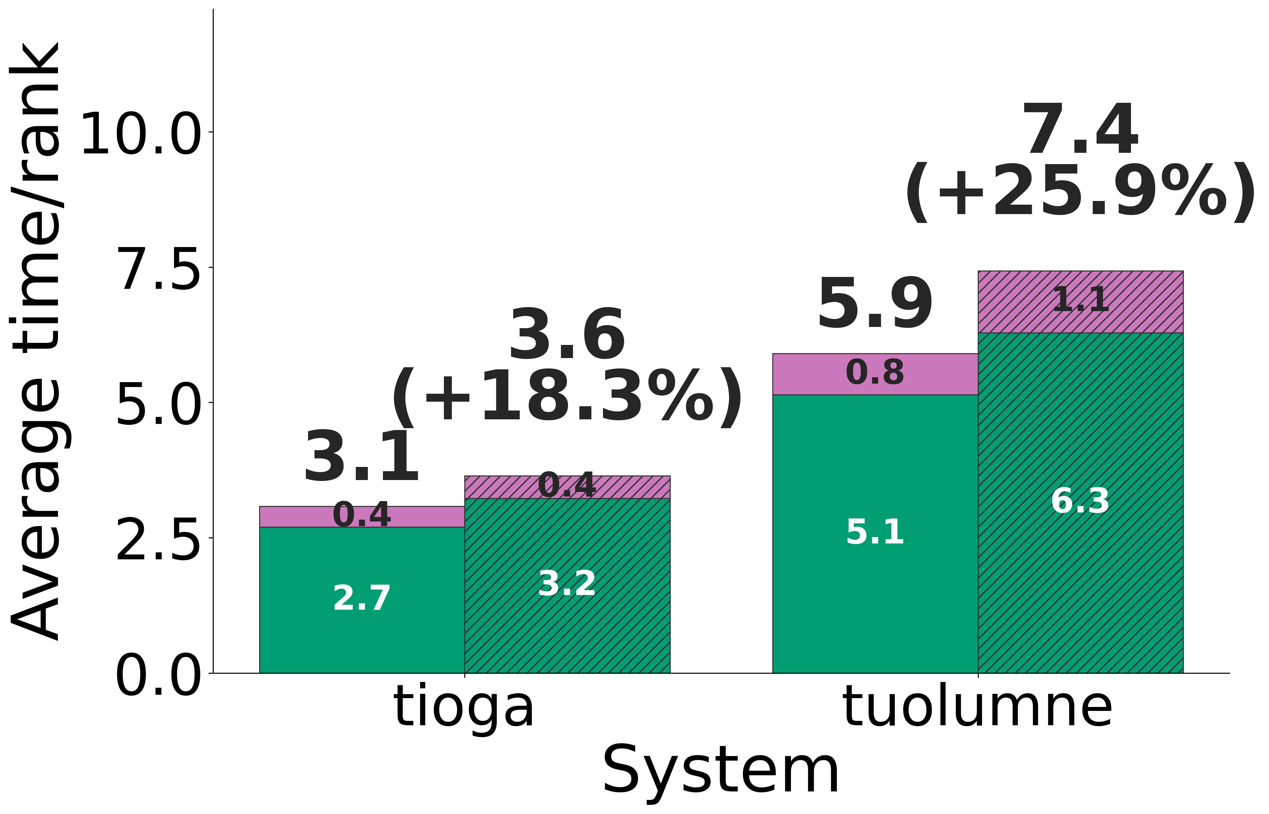
AMG2023 computation and communication time by system and ROCm version.

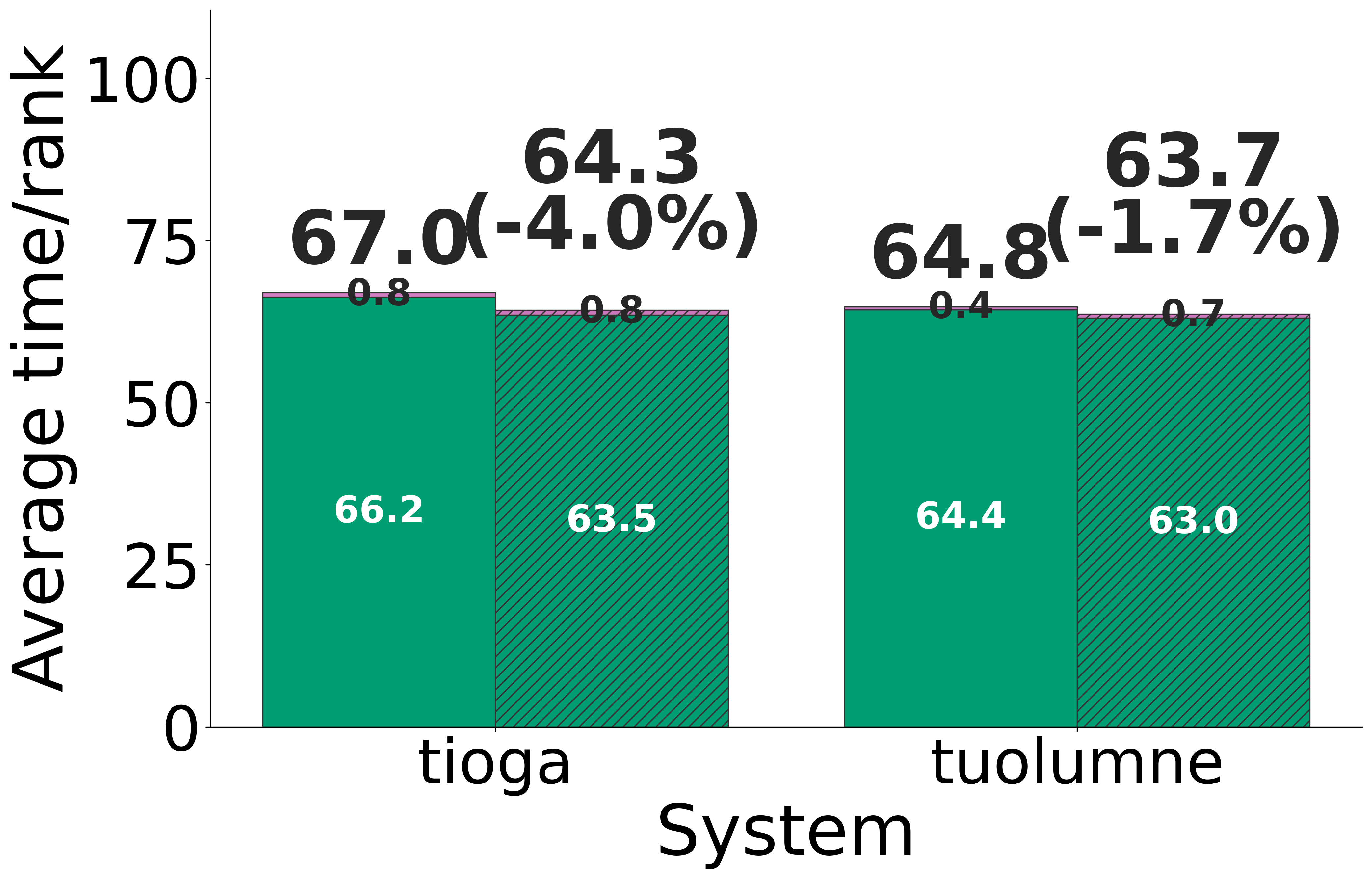
Kripke computation and communication time by system and ROCm version.

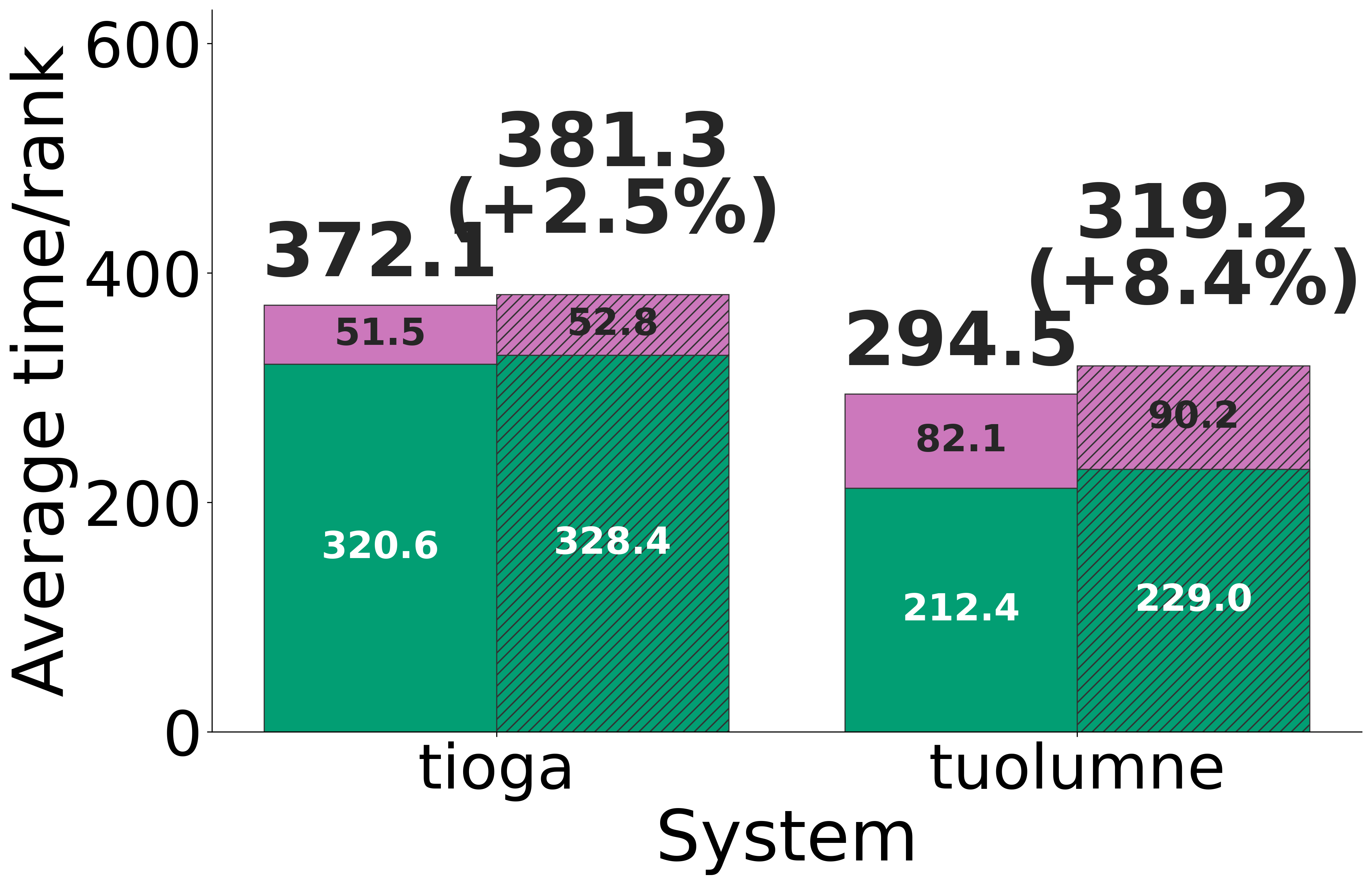
Laghos computation and communication time by system and ROCm version.

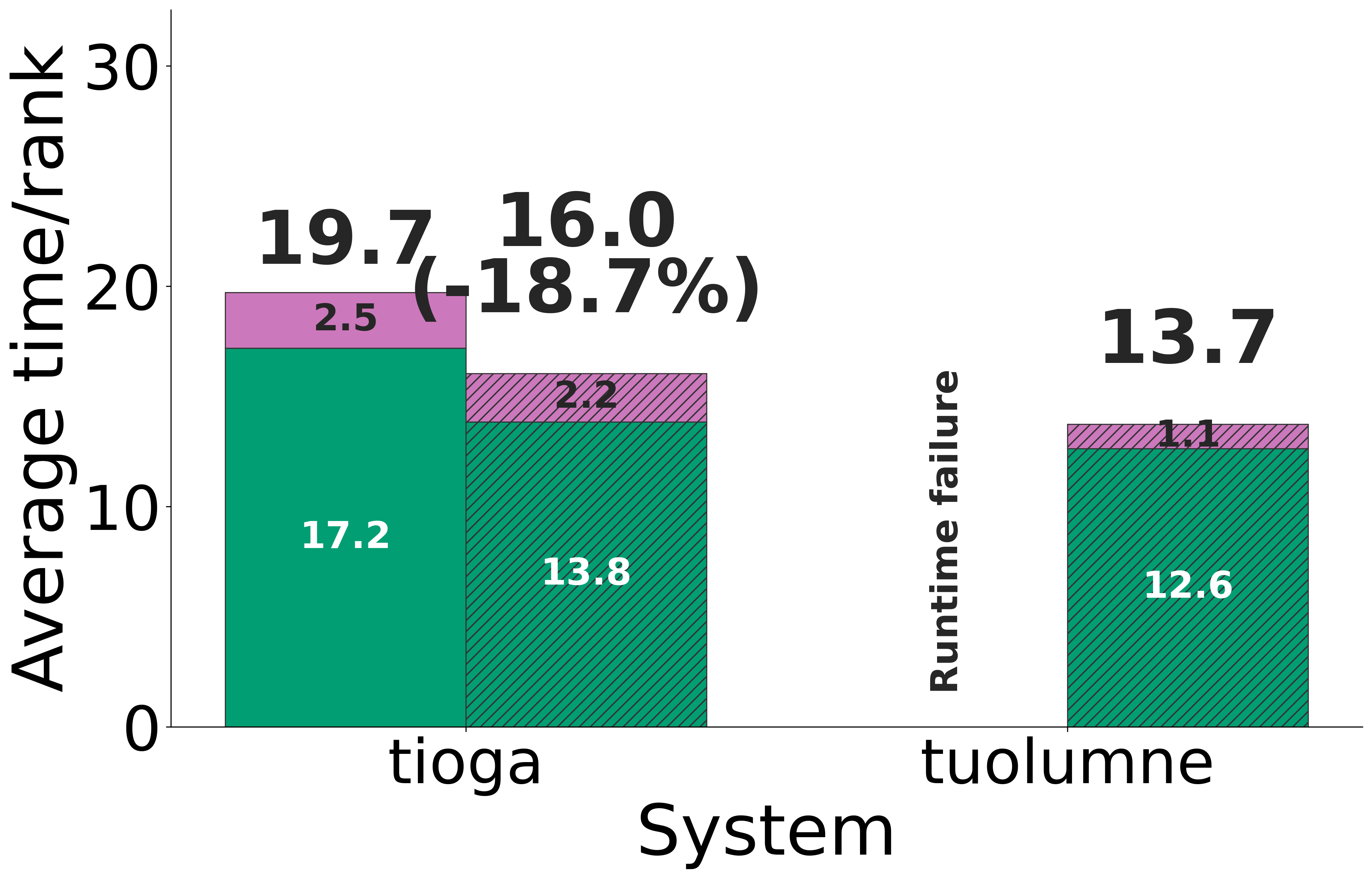
LAMMPS computation and communication time by system and ROCm version.