Analyze a Scaling Study

The benchpark analyze command can be used to generate pre-defined charts for analysis of scaling studies using Caliper and Thicket. The study must use the Caliper modifier caliper=time,mpi (Benchpark Modifiers) to collect the performance data. benchpark analyze uses the Thicket performance analysis library to compose and visualize the Caliper performance data.

benchpark analyze will generate:

1. A calltree of the regions that were executed in the benchmark.

2. A scaling study figure, which can be configured with command-line arguments.

3. A csv of the datapoints plotted on the figure.

benchpark analyze requires additional Python packages, which can be installed by running pip install .[analyze] in the benchpark directory.

To run benchpark analyze:

$ benchpark analyze --workspace-dir RAMBLE_WORKSPACE_DIR <optional_arguments>

benchpark analyze has many options, explained in the help menu for the command.

usage: main.py analyze [-h]

options:
  -h, --help  show this help message and exit

Calltree

We will use one of the experiments available in Benchpark, Kripke, to demonstrate the output of the benchpark analyze command.

The output includes the Calltree of the benchmark:

 main
├─  Generate
│  ├─  MPI_Allreduce
│  ├─  MPI_Comm_split
│  └─  MPI_Scan
├─  MPI_Allreduce
├─  MPI_Bcast
├─  MPI_Comm_dup
├─  MPI_Comm_free
├─  MPI_Comm_split
├─  MPI_Finalize
├─  MPI_Finalized
├─  MPI_Gather
├─  MPI_Get_library_version
├─  MPI_Initialized
└─  Solve
  └─  solve
      ├─  LPlusTimes
      ├─  LTimes
      ├─  Population
      │  └─  MPI_Allreduce
      ├─  Scattering
      ├─  Source
      └─  SweepSolver
        ├─  MPI_Irecv
        ├─  MPI_Isend
        ├─  MPI_Testany
        ├─  MPI_Waitall
        └─  SweepSubdomain

Strong Scaling

To generate a strong scaling dataset, you would need to run the strong scaling scaling study of Kripke:

$ benchpark system init --dest=lassen llnl-sierra
$ benchpark experiment init --dest=kripke/cuda/strong lassen kripke+cuda+strong caliper=time,mpi
$ benchpark setup lassen/kripke/cuda/strong wkp
// Follow instructions for running Ramble ...

Run benchpark analyze:

$ benchpark analyze --workspace-dir wkp/kripke/cuda/strong/lassen/workspace/

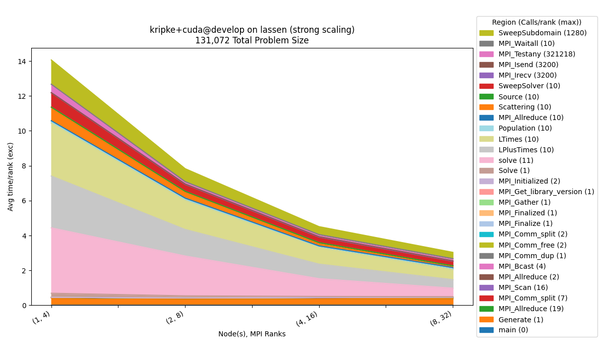
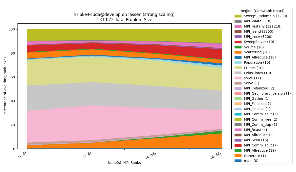
The default configuration will visualize a stacked area chart of:

• The exclusive average time per rank Avg time/rank (exc) collected by the caliper modifier caliper=time.

• Number of nodes and number of MPI ranks on the x-axis, which are the parameters we vary in the experiment (for strong scaling).

• Constant information will be contained in the title, such as benchmark, programming model, benchmark version, cluster, etc.

• The legend will contain the regions and maximum calls out of all of the ranks (Calls/rank (max)).

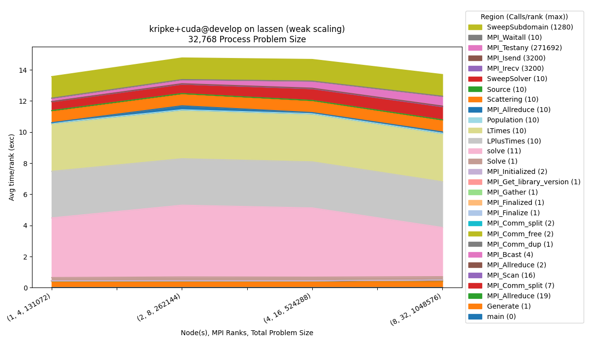
Weak Scaling

To generate the weak scaling dataset:

$ benchpark experiment init --dest=kripke/cuda/weak lassen kripke+cuda+weak caliper=time,mpi
$ benchpark setup lassen/kripke/cuda/weak wkp
// Follow instructions for running Ramble ...

Run benchpark analyze:

$ benchpark analyze --workspace-dir wkp/kripke/cuda/weak/lassen/workspace/

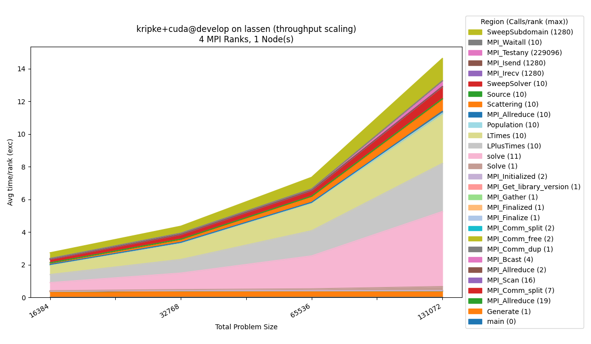
Throughput

To generate the throughput dataset:

$ benchpark experiment init --dest=kripke/cuda/throughput lassen kripke+cuda+throughput caliper=time,mpi
$ benchpark setup lassen/kripke/cuda/throughput wkp
// Follow instructions for running Ramble ...

Run benchpark analyze:

$ benchpark analyze --workspace-dir wkp/kripke/cuda/throughput/lassen/workspace/

Percentage

$ benchpark analyze --workspace-dir wkp/kripke/cuda/strong/lassen/workspace/ --chart-type percentage

The --chart-type percentage option, visualizes the y-axis metric, relative to the summation of the metric for all regions. This is useful in this example to visualize what percentage of the time each region is taking.

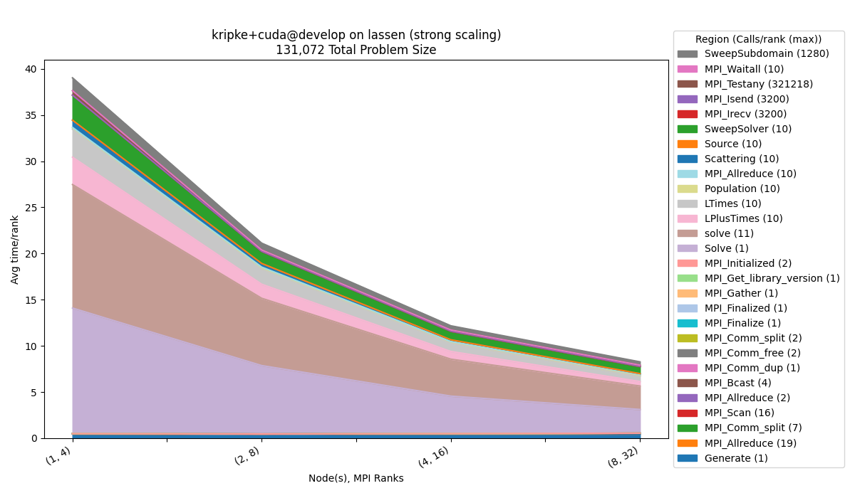
Inclusive Metrics

$ benchpark analyze --workspace-dir wkp/kripke/cuda/strong/lassen/workspace/ --yaxis-metric "Avg time/rank"

We can also visualize any inclusive metrics by selecting them as the yaxis_metric. Here we use Avg time/rank instead of Avg time/rank (exc). The main node is automatically removed from the figure, because this information is redundant for the inclusive metric.

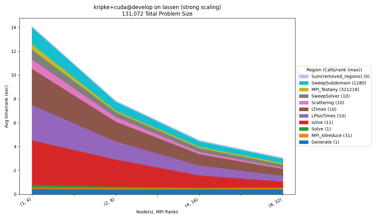
Region Filtering

$ benchpark analyze --workspace-dir wkp/kripke/cuda/strong/lassen/workspace/ --group-regions-name --top-n-regions 10

An efficient way to filter out smaller regions quickly, is to use the --group-regions-name and --top-n-regions parameters. --group-regions-name computes the sum of the metric for all of the regions with the same name, so multiple regions are shown as a single region. --top-n-regions filters the data to only show the n regions with the highest values for the given metric (based on the first profile). We can also add the --no-mpi argument to filter out all MPI_* regions.

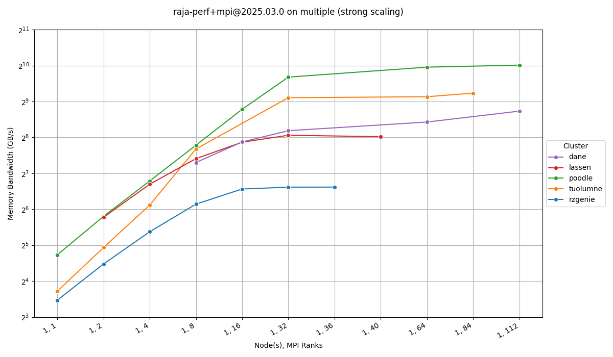
Visualize Data From Multiple Workspaces

Data from multiple clusters will end up in separate Ramble workspaces. Simply point at the Benchpark workspace instead of the Ramble workspace to include multiple Ramble workspaces in your analysis. This example uses the line chart functionality to visualize a single node memory bandwidth study. Other options are bar and scatter.

Note

The area chart will not work for data from multiple Ramble workspaces.

$ benchpark analyze --workspace-dir wkp/ --query-regions-byname Stream_TRIAD --chart-kind line --file-name-match Base_Seq-default --yaxis-metric 'Memory Bandwidth (GB/s)' --chart-yaxis-limits 8 2048 --chart-figsize 12 7 --yaxis-log --no-mpi

Visualize a Metadata Column

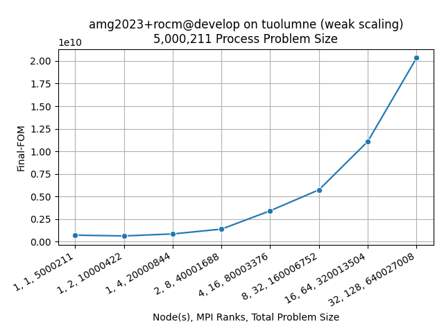
benchpark analyze is not limited to performance data columns. Provide the name of a metadata column to visualize that instead. This is useful for metrics like FOM’s, which only have one value per profile.

$ benchpark analyze --workspace-dir problem1/ --yaxis-metric Final-FOM --chart-kind line --disable-legend