3. RAJA Performance Suite
The RAJA Performance Suite contains a variety of numerical kernels that represent important computational patterns found in HPC applications. It is a companion project to RAJA, which is a library of software abstractions used by developers of C++ applications to write portable, single-source code. Each kernel in the Suite has multiple implementations using common parallel programming models, such as OpenMP and CUDA, including RAJA and non-RAJA (often referred to as Base) variants. The RAJA Performance Suite enables a wide range of performance experiments and comparisons for kernel variants, compilers, etc.
Important
The RAJA Performance Suite Benchmark is limited to a subset of kernels in the RAJA Performance Suite described in Problems.
The RAJAPerf-Benchmark GitHub repo contains the source code, performance baseline data files, run scripts, and data processing scripts for the RAJA Performance Suite Benchmark. It includes the RAJA Performance Suite repo as a submodule which, in turn, contains RAJA as a submodule. When the benchmark project repo is cloned recursively, everything necessary to build and run the benchmark is included. Detailed instructions are included in Building and Running.
Additional information about the RAJA Performance Suite and RAJA is available at these links:
3.1. Purpose
The main purpose of the RAJA Performance Suite is to analyze performance of loop-based computational kernels representative of those found in HPC applications and to compare implementation variants. The kernels in the Suite originate from various sources ranging from open-source HPC benchmarks to restricted-access production applications. Kernels exercise a variety of loop structures and important parallel operations such as reductions, atomics, scans, and sorts.
Each kernel in the Suite appears in RAJA and non-RAJA variants that exercise common programming models, such as OpenMP, CUDA, and HIP. Performance comparisons between RAJA and non-RAJA variants are helpful to improve RAJA implementations and to identify impacts that C++ abstractions have on compilers’ abilities to optimize. The Suite serves as an important collaboration tool between the RAJA team and vendors to resolve performance issues observed in production applications that use RAJA.
3.2. Characteristics
RAJAPerf-Benchmark GitHub repo contains everything needed to build and run the benchmark. This includes the RAJA Performance Suite and RAJA software dependencies in Git submodules and scripts to build, run, and analyze output data. Thus, all dependency versions are pinned to each version of the benchmark. Building the RAJA Performance Suite code requires CMake to configure a build, a C++17 (soon to require C++20) compliant compiler to build the code, and an MPI library installation to link against.
The Suite can be run in a myriad of ways via command-line options and their arguments. The intent is that after compiling the code, simple scripts can be written to execute necessary Suite runs to generate data for desired performance experiments. Instructions for getting the code for the RAJA Performance Suite Benchmark, building it, and running it are described in Building and Running.
3.2.1. Problems
The RAJA Performance Suite Benchmark consists of a subset of kernels in the full Suite that focus on some key computational patterns found in LLNL applications. The benchmark kernels are partitioned into two priority levels as described below, along with notable features and RAJA constructs used in each kernel (in parentheses).
Note
In the RAJA Performance Suite repository, each kernel contains a
detailed reference description near the top of the header file for
the kernel class; i.e., C++ header file named <kernel-name>.hpp.
The reference description is a C-style sequential implementation of
the kernel in a comment section near the top of the file.
The RAJA Performance Suite Benchmark kernels are partitioned into two priority levels described below.
3.2.1.1. Priority 1 kernels
Priority 1 kernels are most important to us. They are located in the
RAJAPerf/src/apps sub-directory:
DIFFUSION3DPA element-wise action of a 3D finite element volume diffusion operator via partial assembly and sum factorization (nested loops, GPU shared memory, RAJA::launch API)
EDGE3D stiffness matrix assembly for a 3D MHD calculation (single loop with included function call, RAJA::forall API)
ENERGY internal energy calculation from an explicit hydrodynamics algorithm; (multiple single-loop operations in sequence, conditional logic for correctness checks and cutoffs, RAJA::forall API)
FEMSWEEP finite element implementation of linear sweep algorithm used in radiation transport, with a register-heavy LU solver (nested loops, RAJA::launch API)
INTSC_HEXRECT intersection between a 24-sided hexahedron and a rectangular solid, including volume and moment calculations (single loop, RAJA::forall API)
MASS3DEA element assembly of a 3D finite element mass matrix (nested loops, GPU shared memory, RAJA::launch API)
MASS3DPA_ATOMIC action of a 3D finite element mass matrix on elements with shared DOFs via partial assembly and sum factorization (nested loops, GPU shared memory, RAJA::launch API)
MASSVEC3DPA element-wise action of a 3D finite element mass matrix via partial assembly and sum factorization on a block vector (nested loops, GPU shared memory, RAJA::launch API)
NODAL_ACCUMULATION_3D on a 3D structured hexahedral mesh, sum a contribution from each hex vertex (nodal value) to its centroid (zonal value) (single loop, data access via indirection array, 8-way atomic contention, RAJA::forall API)
VOL3D on a 3D structured hexahedral mesh (faces are not necessarily planes), compute volume of each zone (hex) (single loop, data access via indirection array, RAJA::forall API)
3.2.1.2. Priority 2 kernels
Priority 2 kernels are also important, but less so than the Priority 1
kernels listed above. Priority 2 kernels are listed below and are located in
the RAJAPerf/src sub-directories noted:
apps/CONVECTION3DPA element-wise action of a 3D finite element volume convection operator via partial assembly and sum factorization (nested loops, GPU shared memory, RAJA::launch API)
apps/DEL_DOT_VEC_2D divergence of a vector field at a set of points on a mesh (single loop, data access via indirection array, RAJA::forall API)
apps/INTSC_HEXHEX intersection between two 24-sided hexahedra, including volume and moment calculations (multiple single-loop operations in sequence, RAJA::forall API)
apps/LTIMES one step of the source-iteration technique for solving the steady-state linear Boltzmann equation, multi-dimensional matrix product (nested loops, RAJA::kernel API)
apps/MASS3DPA element-wise action of a 3D finite element mass matrix via partial assembly and sum factorization (nested loops, GPU shared memory, RAJA::launch API)
apps/MATVEC_3D_STENCIL matrix-vector product based on a 3D mesh stencil (single loop, data access via indirection array, RAJA::forall API)
basic/MULTI_REDUCE multiple reductions in a kernel, where number of reductions is set at run time (single loop, irregular atomic contention, RAJA::forall API)
basic/REDUCE_STRUCT multiple reductions in a kernel, where number of reductions (6) is known at compile time (single loop, multiple reductions, RAJA::forall API)
basic/INDEXLIST_3LOOP construction of set of indices used in other kernel executions (single loops, vendor scan implementations, RAJA::forall API)
comm/HALO_PACKING_FUSED packing and unpacking MPI message buffers for point-to-point distributed memory halo data exchange for mesh-based codes (overhead of launching many small kernels, GPU variants use RAJA::Workgroup concepts to execute multiple kernels with one launch)
3.2.2. Figure of Merit
The figure of merit (FOM) for each kernel is determined by the problem size at which the kernel saturates resources on a single compute node. That is, the problem size at which a computational throughput curve becomes flat, with zero derivative, and beyond which running larger problem sizes does not yield an increase in compute rate. The FOM for each kernel includes 3 numerical values:
the saturation problem size (GB)
the compute rate (GFLOP/sec) at the saturation problem size
the memory bandwidth (GB/sec) at the saturation problem size
Important
In the results presented in Example Benchmark Results, problem size is computed individually for each kernel based on a requested memory allocation size. The concept of size is subjective and depends on what one is looking for. We discuss how we determine problem sizes for the kernels in the RAJA Performance Suite in https://rajaperf.readthedocs.io/en/develop/sphinx/user_guide/output.html#notes-about-problem-size
When the Suite is run, problem size, compute rate, and memory bandwidth, among other data are reported in output files. We provide a Python script that can traverse the contents of an output directory and generate condensed summary files, throughput plots, and FOM information. Usage of the script is detailed below.
Computational throughput may be visualized using a plot where compute rate,
such as GFLOP/sec (vertical axis), is plotted as a function of problem size on
the horizontal axis. Ideally, such a curve will be monotonically
increasing and transition to a flat, horizontal line. Then, the saturation point
is the problem size at which the derivative of the throughput curve becomes zero.
In reality, throughput curves are often non-monotonic or do not have a
strictly zero derivative for all points beyond some problem size. Therefore, we
apply a simple median based smoothing algorithm to the throughput curve data
and heuristically estimate the saturation point based on the smoothed
throughput curve. The details of our approach are documented in the
process_data.py script in the
RAJAPerf-Benchmark GitHub repo,
which we use in Example Benchmark Results
Lastly, we emphasize that we want the kernels to be run in an execution environment that aligns with how they would run if part of a real application. Thus, the Suite should be run using multiple MPI ranks so that all resources on a compute node are being exercised in a way that is representative of how an application would run.
All applications that use RAJA use it in the MPI + X parallel application paradigm, where MPI is used for coarse-grained, distributed memory parallelism and X (RAJA in this case) supports fine-grained parallelism within each MPI rank. The RAJA Performance Suite can be configured with MPI so that execution of kernels in the Suite follows the MPI + X application paradigm. When a kernel is run using multiple MPI ranks, the same code executes simultaneously on each, and synchronization and communication among ranks involves only the sending execution timing information from each rank to rank zero for reporting purposes.
Important
For RAJA Performance Suite benchmark execution, MPI must be used to run to ensure that all resources on a compute node are being exercised so as to avoid misrepresentation of kernel and node performance. This is described in Running.
3.3. Source code modifications
Please see Run Rules Synopsis for general guidance on allowed modifications. For the RAJA Performance Suite, we define the following restrictions on source code modifications:
While source code changes to the RAJA Performance Suite kernels and to RAJA can be proposed for improved performance, for example, RAJA may not be removed from RAJA kernel variants in the Suite or replaced with any other library. The non-RAJA kernel variants in the Suite are provided to show how each kernel can be implemented directly in the corresponding programming model back-end without the RAJA abstraction layer. Apart from some special cases, the RAJA and non-RAJA variants for each kernel should execute the same operations.
3.4. Building
3.4.1. Getting the code
All non-system related software dependencies needed to compile and run the
benchmark are contained in the
RAJAPerf-Benchmark GitHub repo
repository as Git submodules. The v2026.04.1 version of the repo is the
current version and was used to generate the baseline data described in
Example Benchmark Results.
The following command can be used to clone the GitHub repo:
$ git clone --recursive git@github.com:llnl/RAJAPerf-Benchmark.git
This will clone the repo into your local directory and put you on the main
branch of the benchmark repo, which is the default branch. To get a local copy
of the version used to generate the baselines, execute the following commands:
$ git checkout v2026.04.1
$ git submodule update --init --recursive
This will assure that you have the proper versions of the RAJAPerf and RAJA submodules in your repo clone.
3.4.2. Configuration and compilation
The RAJA Performance Suite uses a CMake-based system to configure the code for compilation. When building the RAJA Performance Suite, RAJA and the RAJA Performance Suite are built together with the same CMake configuration which is specified at the RAJA Performance Suite level. The generic process for specifying a configuration and generating a build space is to create a build directory and run CMake in it with the proper options. For example:
$ pwd
path/to/RAJAPerf
$ mkdir my-build
$ cd my-build
$ cmake <cmake args> ..
$ make -j (or make -j <N> to build with a specified number of cores)
For convenience and informational purposes, we maintain configuration scripts
in RAJAPerf/scripts subdirectories for various builds. For example, the
RAJAPerf/scripts/lc-builds directory contains scripts that we use to
generate build configurations for machines in the Livermore Computing (LC)
Center at Lawrence Livermore National Laboratory for basic development.
These scripts are run in the top-level RAJAPerf directory. Each script creates
a descriptively-named build space directory and runs CMake to generate a build
space appropriate for the
platform and compiler(s) indicated by the script name and arguments passed to
it. Executing a script with no arguments will print a message indicating
which arguments are required.
3.4.3. MI300A architecture
To configure and build the code to generate baseline data on a system with AMD MI300A processors (i.e., ATS-4 (El Capitan) architecture) discussed in Example Benchmark Results, we ran the following commands:
$ pwd
path/to/RAJAPerf
$ ./scripts/lc-builds/toss4_cray-mpich_amdclang.sh 9.0.1 6.4.3 gfx942
$ cd build_lc_toss4-cray-mpich-9.0.1-amdclang-6.4.3-gfx942
$ make -j
Specifically, we configured and compiled the code for execution using version 9.0.1 of the Cray MPICH MPI library and the AMD clang compiler with ROCm version 6.4.3 targeting GPU compute architecture gfx942.
3.4.4. H100 architecture
To configure and build the code to generate baseline data on a system with NVIDIA H100 processors discussed in Example Benchmark Results, we ran the following commands:
$ pwd
path/to/RAJAPerf
$ ./scripts/lc-builds/toss4_mvapich2_nvcc_gcc.sh 2.3.7 12.9.1 90 10.3.1
$ cd build_lc_toss4-mvapich2-2.3.7-nvcc-12.9.1-90-gcc-10.3.1
$ make -j
Specifically, we configured and compiled the code for execution using version 2.3.7 of the MVAPICH2 MPI library, version 12.9.1 of the nvcc compiler for CUDA targeting GPU compute architecture sm_90, and version 10.3.1 of the GNU compiler for compiling host code.
3.5. Running
After the RAJA Performance Suite code is built, the executable will be located
in the bin subdirectory of the build space.
To get information about how to run the code, use the help option:
$ pwd
path/to/RAJAPerf
$ cd my-build
$ ls bin
raja-perf.exe
$ ./bin/raja-perf.exe --help (or -h)
This will print all available command-line options along with potential arguments and defaults. Available options allow one to print information about the kernels in the Suite, to select output directory and file details, to select kernels and variants to run, to define how kernels are run (problem sizes, # times each kernel is run to collect min/max/avg timing data, data spaces to use for array allocation, etc.). All arguments are optional. If no arguments are specified, the suite will run all kernels in their default configurations for the variants that are available based on the way the code was compiled.
In Example Benchmark Results, we provide the exact commands we used to run the code and generate the baseline results for the benchmark.
3.6. Validation
Each kernel variant run generates a checksum value based on the result of its execution, such as an output data array computed by the kernel. The checksum depends on the problem size run for the kernel; thus, each checksum is computed at run time. Validation criteria are defined in terms of the checksum difference between each kernel variant and problem size run and a corresponding reference variant. The reference variant is the baseline sequential (CPU) variant for each kernel. The run scripts, described below, execute the baseline sequential variant in addition to the benchmark variants to validate the answers of the benchmark variants.
Each kernel is annotated in the source code as to whether the checksum for
each variant is expected to match the reference checksum exactly, or to be
within some tolerance due to order of operation or other differences when run in
parallel. Whether the checksum for a kernel is within its expected tolerance
is reported as checksum PASSED or FAILED in the checksum output files.
3.7. Example Benchmark Results
As stated earlier, we are mainly interested in single-node performance
with this benchmark. To generate throughput curves and estimate
saturation points, we use a bash shell script to run the code on each
platform and a Python script to process the data to construct throughput
plots, estimate saturation points, and make CSV files for tables of results.
These scripts are also available in the
RAJAPerf-Benchmark GitHub repo.
The scripts and results discussed here are located in the scripts/2026-FCR
directory there.
Important
In the following sections, we present detailed results, including FOM tables and throughput plots for the Priority 1 kernels described above. For completeness, we also include a brief summary of results for Priority 2 kernels in less detail. Data files containing results for all kernels run are included in this repository.
3.7.1. AMD MI300A throughput results (Priority 1 kernels)
For the MI300A architecture, we present two sets of throughput results. One is
run in SPX mode where we use 4 MPI ranks on a node, one for each MI300A APU,
and treat each APU as a single GPU. The other is run in
CPX mode where we run with 24 MPI ranks on a node, six for each MI300A
APU, and treat each APU as 6 GPUs (one GPU = 1 XCD). In each case, we run
each kernel over a sequence of problem sizes such that the saturation point is
evident on its associated throughput curve.
3.7.1.1. SPX mode (Priority 1)
For SPX mode (run with 1 MPI rank per APU on a node), we choose the smallest problem to use ~100,000 bytes of allocated memory and the largest problem to use ~400MB of allocated memory, which is about 1.5 times the MALL (Memory Attached Last-Level cache) size on the MI300A. The MALL is 256 MB (256 * 1024 * 1024 = 268435456 bytes).
Note that for two of the kernels FEMSWEEP and MASS3DEA, we ran a
different problem size range because these kernels don’t clearly saturate.
For them, we chose the smallest problem to use ~3.2MB of allocated
memory and the largest problem to use ~600MB memory, which is over twice as
large as the MALL.
After building the code as described in MI300A architecture, we
run the Priority 1 kernels in SPX mode as follows:
$ pwd
path/to/RAJAPerf
$ cd build_lc_toss4-cray-mpich-9.0.1-amdclang-6.4.3-gfx942
$ ./run_tier_mi300a.sh spx tier1
This generates a directory named RPBenchmark_MI300A_tier1-SPX, which
contains the results files for each kernel run over its range of problem sizes.
Then, we process the data for reporting the results in a concise form by running a Python script we provide:
$ pwd
path/to/RAJAPerf
$ python3 path/to/process_data.py --root-dir path/to/build_lc_toss4-cray-mpich-9.0.1-amdclang-6.4.3-gfx942/RPBenchmark_MI300A_tier1-SPX --output-dir path/to/build_lc_toss4-cray-mpich-9.0.1-amdclang-6.4.3-gfx942/RPBenchmark_MI300A_tier1-SPX/Output
This generates throughput curve files for Base_HIP and RAJA_HIP
variants of each kernel and summarizes the FOM (described in
Figure of Merit) in a CSV file. These files will be located in the
directory specified via the --output-dir option above. We include
the files generated by the process_data.py script in this repo in the
directory ./docs/13_rajaperf/baseline_data/RPBenchmark_MI300A_tier1-SPX.
Kernel |
Sat Problem Size |
Sat GFLOP/s |
Sat B/W (GiB per sec.) |
|---|---|---|---|
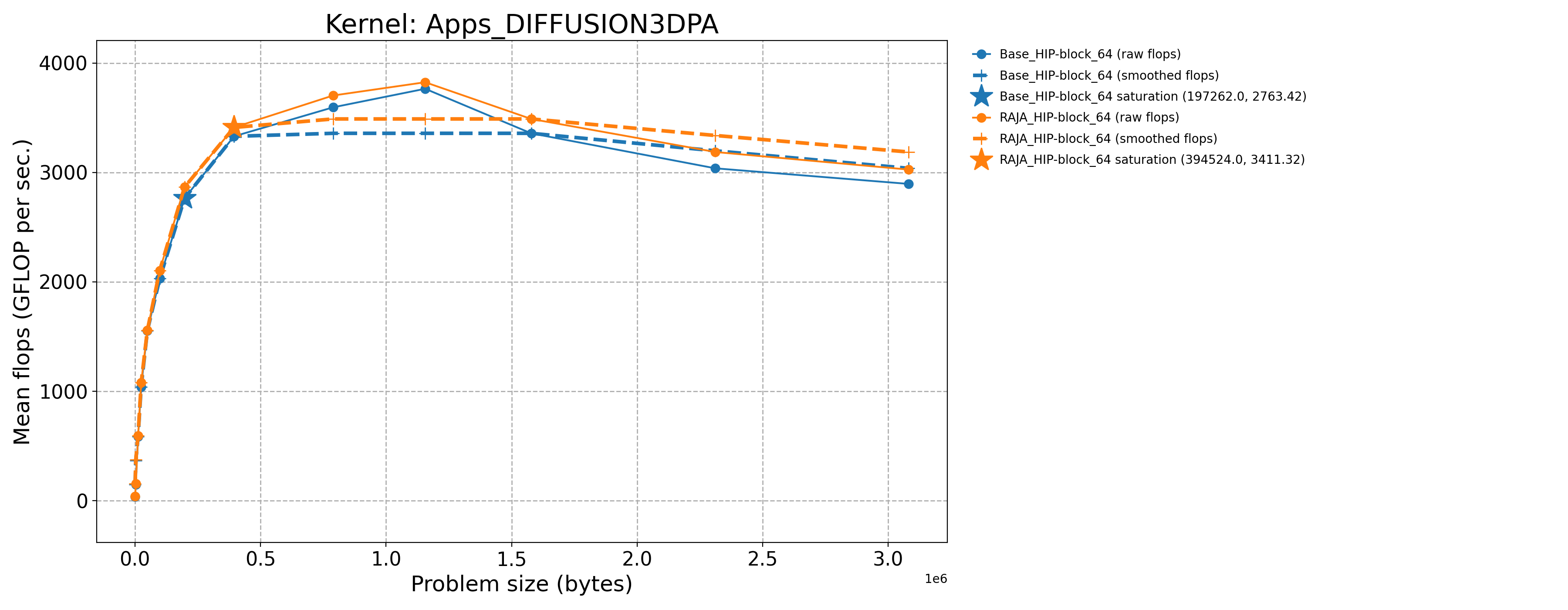
Apps_DIFFUSION3DPA-Base_HIP-block_64 |
197262.0 |
2763.42 |
1841.5 |
Apps_DIFFUSION3DPA-Base_Seq-default |
783.0 |
9.8788 |
6.59477 |
Apps_DIFFUSION3DPA-RAJA_HIP-block_64 |
394524.0 |
3411.32 |
2273.25 |
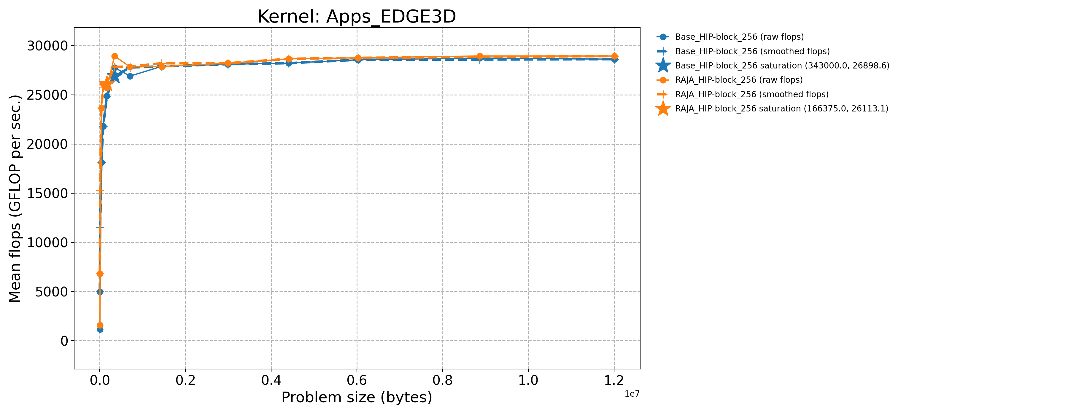
Apps_EDGE3D-Base_HIP-block_256 |
343000.0 |
27771.5 |
63.2963 |
Apps_EDGE3D-Base_Seq-default |
1331.0 |
8.36483 |
0.0200444 |
Apps_EDGE3D-RAJA_HIP-block_256 |
166375.0 |
25705.7 |
58.752 |
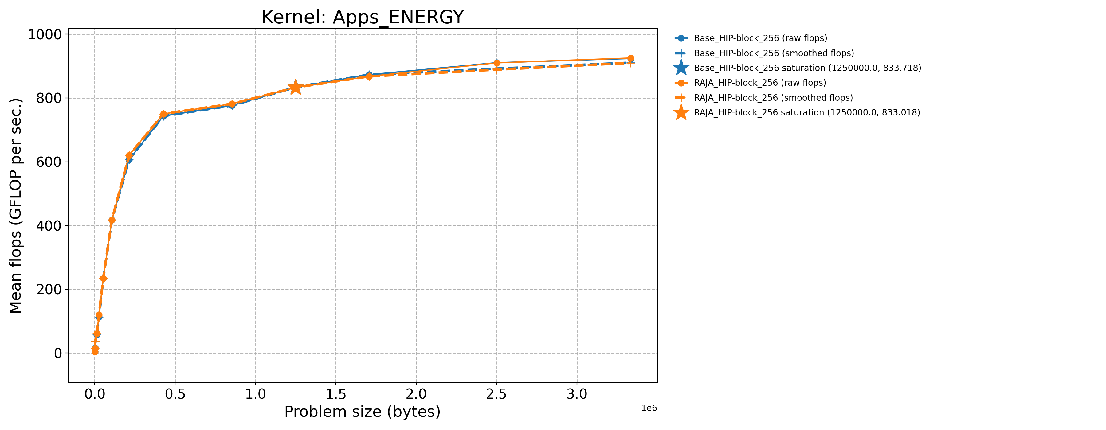
Apps_ENERGY-Base_HIP-block_256 |
1250000.0 |
833.718 |
3049.37 |
Apps_ENERGY-Base_Seq-default |
834.0 |
11.0692 |
40.4861 |
Apps_ENERGY-RAJA_HIP-block_256 |
1250000.0 |
833.018 |
3046.81 |
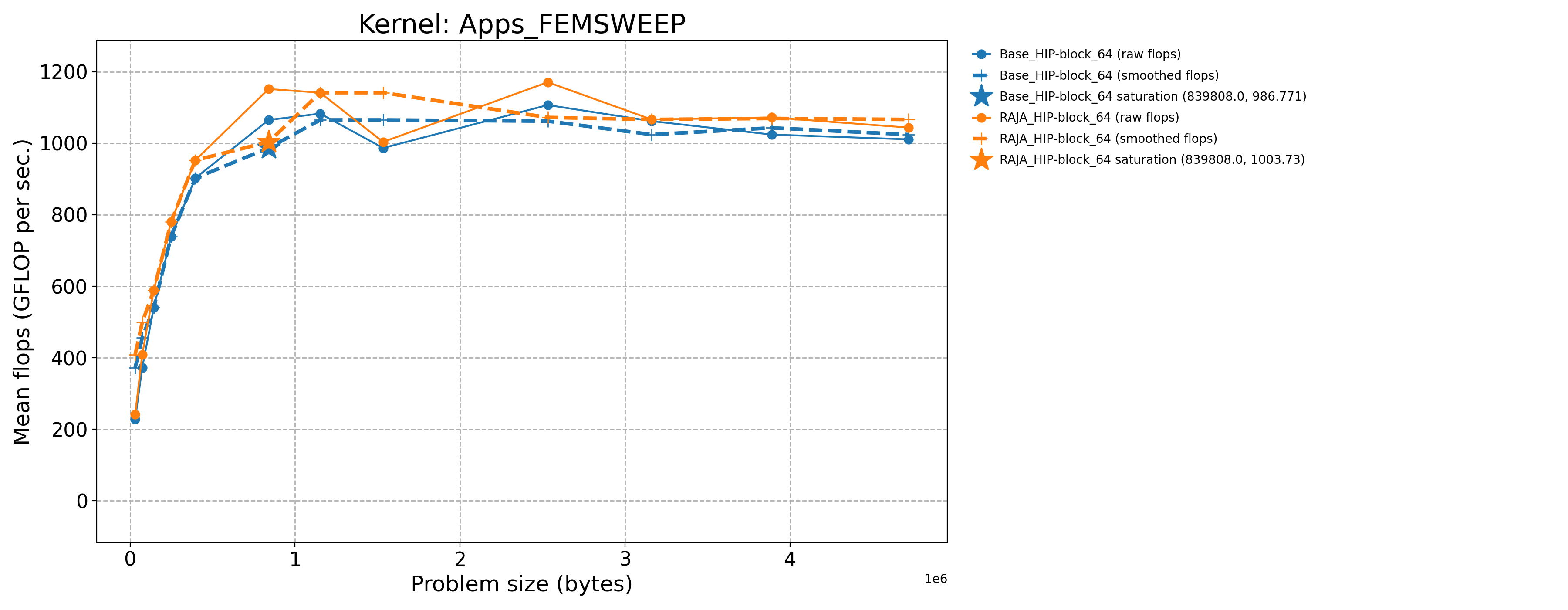
Apps_FEMSWEEP-Base_HIP-block_64 |
839808.0 |
1065.19 |
205.115 |
Apps_FEMSWEEP-Base_Seq-default |
31104.0 |
3.01734 |
0.541864 |
Apps_FEMSWEEP-RAJA_HIP-block_64 |
839808.0 |
1151.79 |
221.79 |
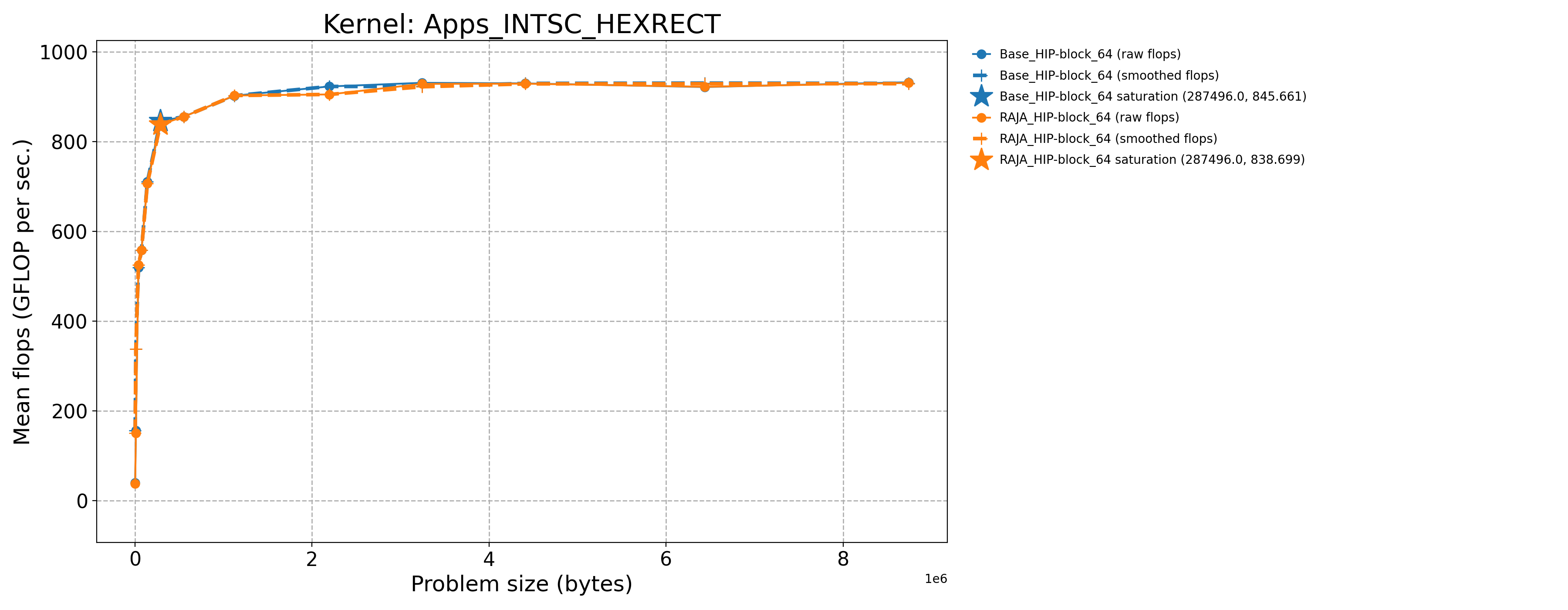
Apps_INTSC_HEXRECT-Base_HIP-block_64 |
287496.0 |
845.661 |
10.3438 |
Apps_INTSC_HEXRECT-Base_Seq-default |
2744.0 |
4.15467 |
0.0521051 |
Apps_INTSC_HEXRECT-RAJA_HIP-block_64 |
287496.0 |
838.699 |
10.2587 |
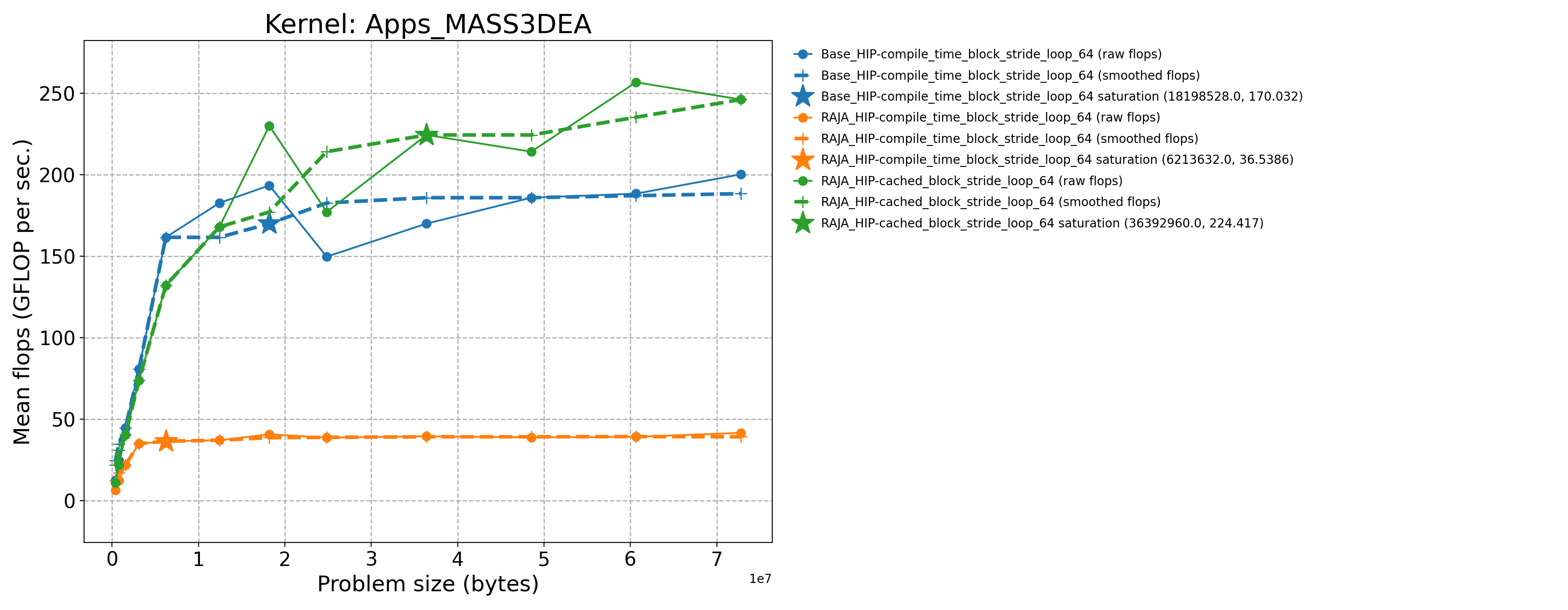
Apps_MASS3DEA-Base_HIP-compile_time_block_stride_loop_64 |
18198528.0 |
193.453 |
212.19 |
Apps_MASS3DEA-Base_Seq-default |
389120.0 |
0.0806808 |
0.0884992 |
Apps_MASS3DEA-RAJA_HIP-cached_block_stride_loop_64 |
36392960.0 |
224.417 |
246.152 |
Apps_MASS3DEA-RAJA_HIP-compile_time_block_stride_loop_64 |
6213632.0 |
36.5386 |
40.0775 |
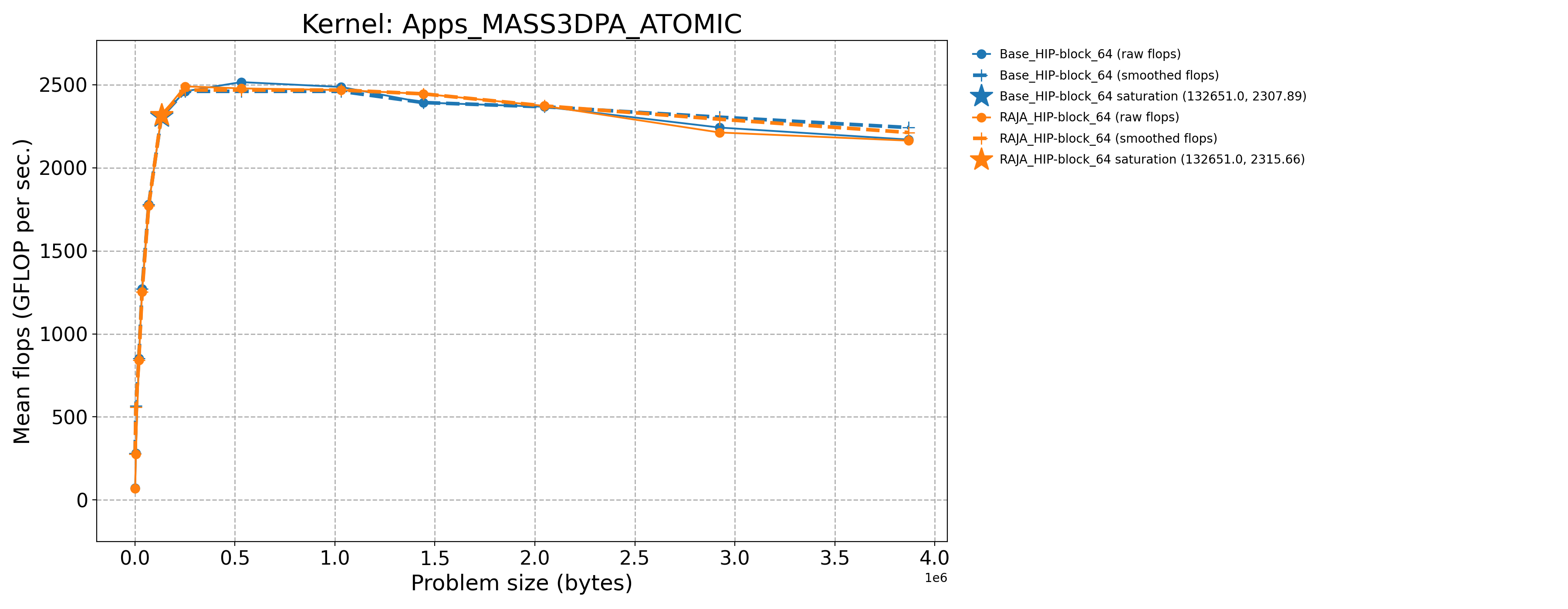
Apps_MASS3DPA_ATOMIC-Base_HIP-block_64 |
132651.0 |
2307.89 |
1072.69 |
Apps_MASS3DPA_ATOMIC-Base_Seq-default |
1331.0 |
10.3068 |
5.06074 |
Apps_MASS3DPA_ATOMIC-RAJA_HIP-block_64 |
132651.0 |
2315.66 |
1076.3 |
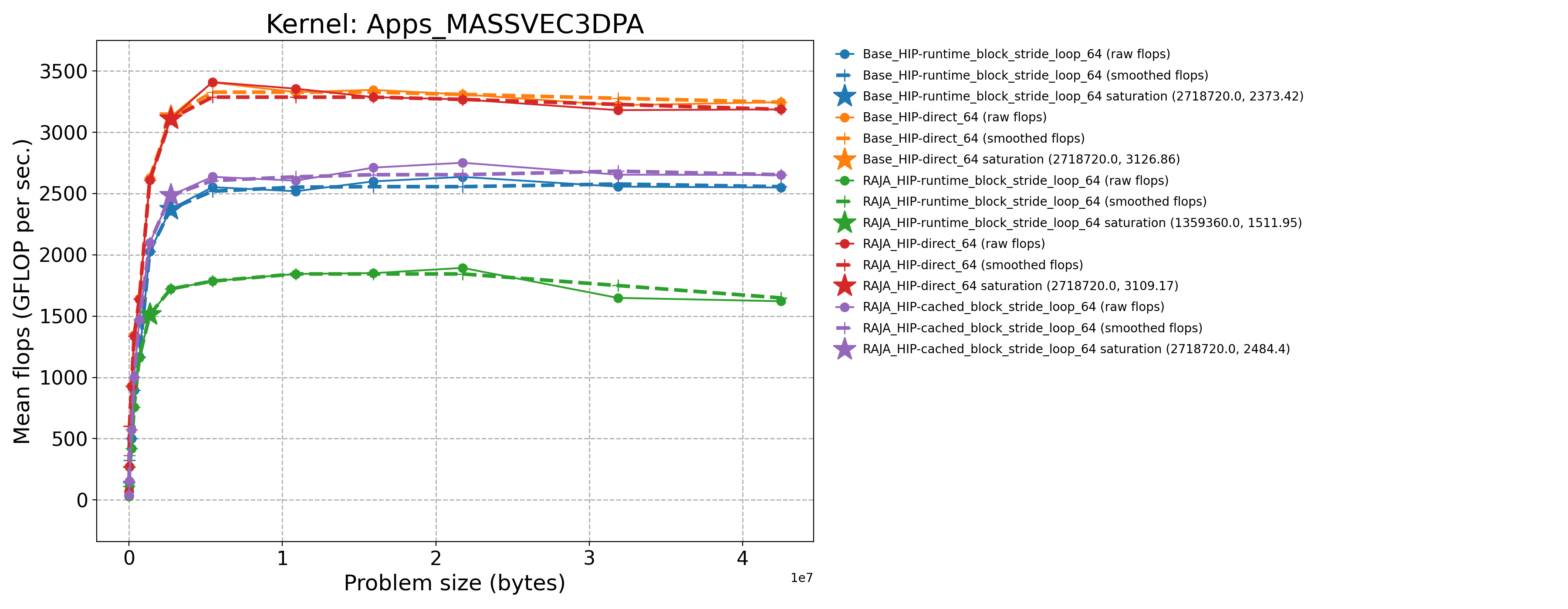
Apps_MASSVEC3DPA-Base_HIP-direct_64 |
2718720.0 |
3126.86 |
953.827 |
Apps_MASSVEC3DPA-Base_HIP-runtime_block_stride_loop_64 |
2718720.0 |
2373.42 |
723.994 |
Apps_MASSVEC3DPA-Base_Seq-default |
10752.0 |
10.98 |
3.35254 |
Apps_MASSVEC3DPA-RAJA_HIP-cached_block_stride_loop_64 |
2718720.0 |
2484.4 |
757.849 |
Apps_MASSVEC3DPA-RAJA_HIP-direct_64 |
2718720.0 |
3109.17 |
948.432 |
Apps_MASSVEC3DPA-RAJA_HIP-runtime_block_stride_loop_64 |
1359360.0 |
1511.95 |
461.21 |
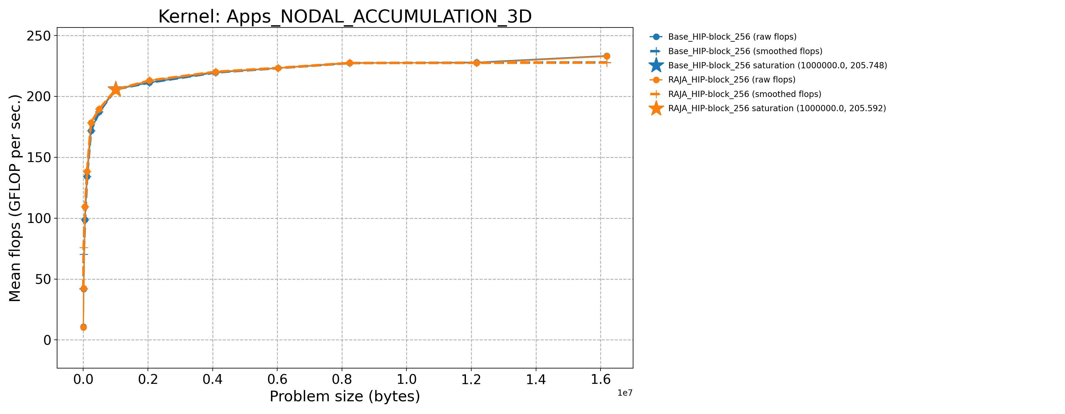
Apps_NODAL_ACCUMULATION_3D-Base_HIP-block_256 |
1000000.0 |
205.748 |
691.63 |
Apps_NODAL_ACCUMULATION_3D-Base_Seq-default |
2744.0 |
1.39555 |
5.1525 |
Apps_NODAL_ACCUMULATION_3D-RAJA_HIP-block_256 |
1000000.0 |
205.592 |
691.105 |
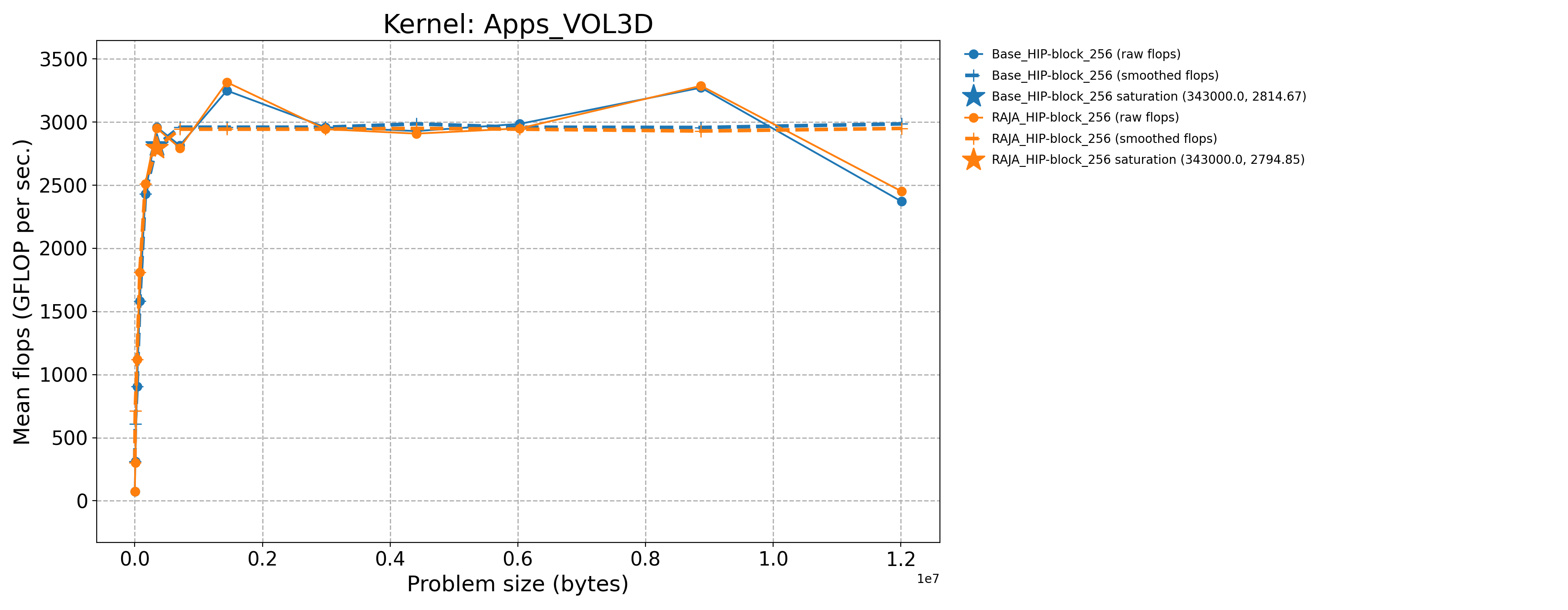
Apps_VOL3D-Base_HIP-block_256 |
343000.0 |
2960.57 |
1238.39 |
Apps_VOL3D-Base_Seq-default |
1331.0 |
16.0597 |
7.06277 |
Apps_VOL3D-RAJA_HIP-block_256 |
343000.0 |
2952.54 |
1235.03 |
3.7.1.2. SPX mode (Priority 2)
The process for generating results for the Priority 2 kernels is essentially
the same as for the Priority 1 kernels just described. Note that two of the
kernels INDEXLIST_3LOOP and HALO_PACKING_FUSED do not perform any
floating point operations. They represent recurring computational patterns
in our application that are important rather than key numerical kernels.
Thus, the two kernels have zero GFLOP/sec rates. So, we consider the bandwidth
as the appropriate metric to consider.
Kernel |
Sat Problem Size |
Sat GFLOP/s |
Sat B/W (GiB per sec.) |
|---|---|---|---|
Apps_CONVECTION3DPA-Base_HIP-block_64 |
351216.0 |
2157.11 |
1191.32 |
Apps_CONVECTION3DPA-Base_Seq-default |
1377.0 |
13.9092 |
7.70152 |
Apps_CONVECTION3DPA-RAJA_HIP-block_64 |
351216.0 |
2159.83 |
1192.82 |
Apps_DEL_DOT_VEC_2D-Base_HIP-block_256 |
264196.0 |
2080.76 |
1727.01 |
Apps_DEL_DOT_VEC_2D-Base_Seq-default |
1849.0 |
8.22078 |
7.01899 |
Apps_DEL_DOT_VEC_2D-RAJA_HIP-block_256 |
528529.0 |
2020.53 |
1675.75 |
Apps_INTSC_HEXHEX-Base_HIP-block_64 |
1728.0 |
19.161 |
0.41308 |
Apps_INTSC_HEXHEX-Base_Seq-default |
27.0 |
3.53728 |
0.0762581 |
Apps_INTSC_HEXHEX-RAJA_HIP-block_64 |
3375.0 |
34.8353 |
0.750994 |
Apps_LTIMES-Base_HIP-block_256 |
619392.0 |
638.563 |
888.12 |
Apps_LTIMES-Base_Seq-default |
2496.0 |
6.38293 |
8.93438 |
Apps_LTIMES-RAJA_HIP-kernel_256 |
619392.0 |
534.613 |
743.546 |
Apps_LTIMES-RAJA_HIP-launch_256 |
619392.0 |
631.91 |
878.867 |
Apps_MASS3DPA-Base_HIP-block_25 |
1619008.0 |
2529.48 |
1178.58 |
Apps_MASS3DPA-Base_Seq-default |
3200.0 |
11.2571 |
5.25832 |
Apps_MASS3DPA-RAJA_HIP-block_25 |
1619008.0 |
2546.38 |
1186.46 |
Apps_MATVEC_3D_STENCIL-Base_HIP-block_256 |
157464.0 |
818.182 |
2025.36 |
Apps_MATVEC_3D_STENCIL-Base_Seq-default |
216.0 |
4.83791 |
15.2267 |
Apps_MATVEC_3D_STENCIL-RAJA_HIP-block_256 |
79507.0 |
699.638 |
1747.18 |
Basic_INDEXLIST_3LOOP-Base_HIP-block_256 |
160000.0 |
0.0 |
282.038 |
Basic_INDEXLIST_3LOOP-Base_Seq-default |
160000.0 |
0.0 |
10.9259 |
Basic_INDEXLIST_3LOOP-RAJA_HIP-block_256 |
160000.0 |
0.0 |
281.64 |
Basic_MULTI_REDUCE-Base_HIP-atomic_direct_256 |
6399995.0 |
171.536 |
2556.08 |
Basic_MULTI_REDUCE-Base_HIP-atomic_occgs_256 |
9374995.0 |
193.002 |
2875.96 |
Basic_MULTI_REDUCE-Base_Seq-default |
6245.0 |
0.314624 |
4.69577 |
Basic_MULTI_REDUCE-RAJA_HIP-atomic_direct_256 |
6399995.0 |
157.081 |
2340.7 |
Basic_MULTI_REDUCE-RAJA_HIP-atomic_occgs_256 |
9374995.0 |
190.404 |
2837.25 |
Basic_REDUCE_STRUCT-Base_HIP-blkatm_direct_256 |
200000.0 |
4.22656 |
31.4902 |
Basic_REDUCE_STRUCT-Base_HIP-blkatm_occgs_256 |
18750000.0 |
144.703 |
1078.12 |
Basic_REDUCE_STRUCT-Base_Seq-cascade |
6250.0 |
1.24252 |
9.25599 |
Basic_REDUCE_STRUCT-Base_Seq-default |
6250.0 |
2.40431 |
17.9107 |
Basic_REDUCE_STRUCT-Base_Seq-kahan |
6250.0 |
0.614436 |
4.57718 |
Basic_REDUCE_STRUCT-RAJA_HIP-blkatm_direct_256 |
6400000.0 |
55.167 |
411.026 |
Basic_REDUCE_STRUCT-RAJA_HIP-blkatm_occgs_256 |
9375000.0 |
270.833 |
2017.87 |
Basic_REDUCE_STRUCT-RAJA_HIP-blkdev_direct_256 |
6400000.0 |
48.8176 |
363.719 |
Basic_REDUCE_STRUCT-RAJA_HIP-blkdev_direct_new_256 |
200000.0 |
2.83301 |
21.1074 |
Basic_REDUCE_STRUCT-RAJA_HIP-blkdev_occgs_256 |
9375000.0 |
257.118 |
1915.68 |
Basic_REDUCE_STRUCT-RAJA_HIP-blkdev_occgs_new_256 |
18750000.0 |
90.5263 |
674.473 |
Comm_HALO_PACKING_FUSED-Base_HIP-direct_1024 |
91125.0 |
0.0 |
53.049 |
Comm_HALO_PACKING_FUSED-Base_Seq-direct |
91125.0 |
0.0 |
30.503 |
Comm_HALO_PACKING_FUSED-RAJA_HIP-direct_1024 |
91125.0 |
0.0 |
43.7518 |
Comm_HALO_PACKING_FUSED-RAJA_HIP-funcptr_1024 |
91125.0 |
0.0 |
46.6773 |
Comm_HALO_PACKING_FUSED-RAJA_HIP-virtfunc_1024 |
91125.0 |
0.0 |
45.935 |
The baseline data files for Priority 2 kernels run on the MI300A architecture in
SPX mode are in this repo in the directory ./docs/13_rajaperf/baseline_data/RPBenchmark_MI300A_tier1-SPX.
3.7.1.3. CPX mode (Priority 1)
For CPX mode (run with 6 MPI ranks per APU on a node), we choose the smallest problem to use ~50,000 bytes of allocated memory and the largest problem to use ~75MB of allocated memory, which is slightly less than 1/3 the MALL size.
Note that for two of the kernels FEMSWEEP and MASS3DEA, we ran a
different problem size range because these kernels don’t clearly saturate.
For them, we chose the smallest problem to use ~1.6MB of allocated
memory and the largest problem to use ~200MB memory, which is a little less
than the MALL size.
Similar to the SPX mode description above, we run the Priority 1 kernels in
CPX mode as follows:
$ pwd
path/to/RAJAPerf
$ cd build_lc_toss4-cray-mpich-9.0.1-amdclang-6.4.3-gfx942
$ ./run_tier_mi300a.sh cpx tier1
This generates a directory named RPBenchmark_MI300A_tier1-CPX, which
contains all the results files for each kernel run over its range of problem
sizes.
Then, we process the data for reporting the results here in a concise form by running a Python script we provide:
$ pwd
path/to/RAJAPerf
$ python3 path/to/process_data.py --root-dir path/to/build_lc_toss4-cray-mpich-9.0.1-amdclang-6.4.3-gfx942/RPBenchmark_MI300A_tier1-CPX --output-dir path/to/build_lc_toss4-cray-mpich-9.0.1-amdclang-6.4.3-gfx942/RPBenchmark_MI300A_tier1-CPX/Output
This generates throughput curve files for Base_HIP and RAJA_HIP
variants of each kernel and summarizes the FOM (described in
Figure of Merit) in a CSV file. These files will be located in the
directory specified by via the --output-dir option above. We include
the files generated by the process_data.py script in this repo in the
directory ./docs/13_rajaperf/baseline_data/RPBenchmark_MI300A_tier1-CPX.
Kernel |
Sat Problem Size |
Sat GFLOP/s |
Sat B/W (GiB per sec.) |
|---|---|---|---|
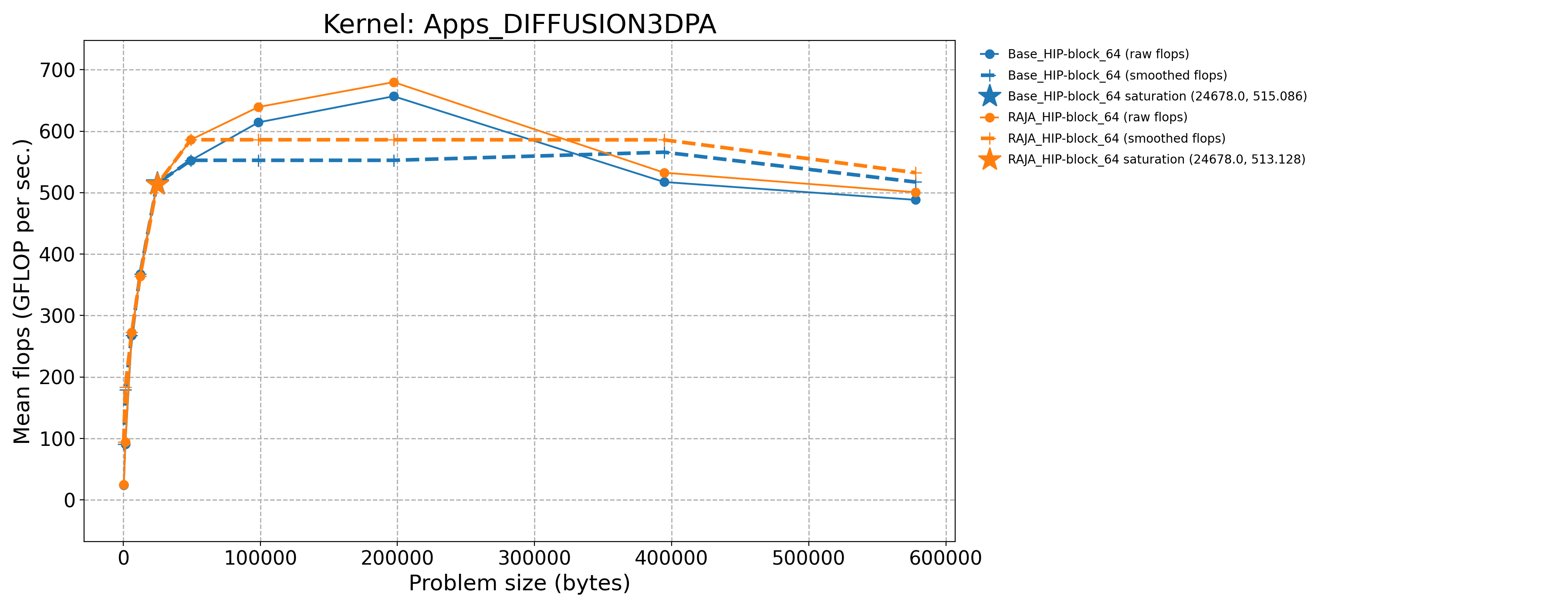
Apps_DIFFUSION3DPA-Base_HIP-block_64 |
24678.0 |
515.086 |
343.264 |
Apps_DIFFUSION3DPA-Base_Seq-default |
405.0 |
9.68515 |
6.47622 |
Apps_DIFFUSION3DPA-RAJA_HIP-block_64 |
24678.0 |
513.128 |
341.959 |
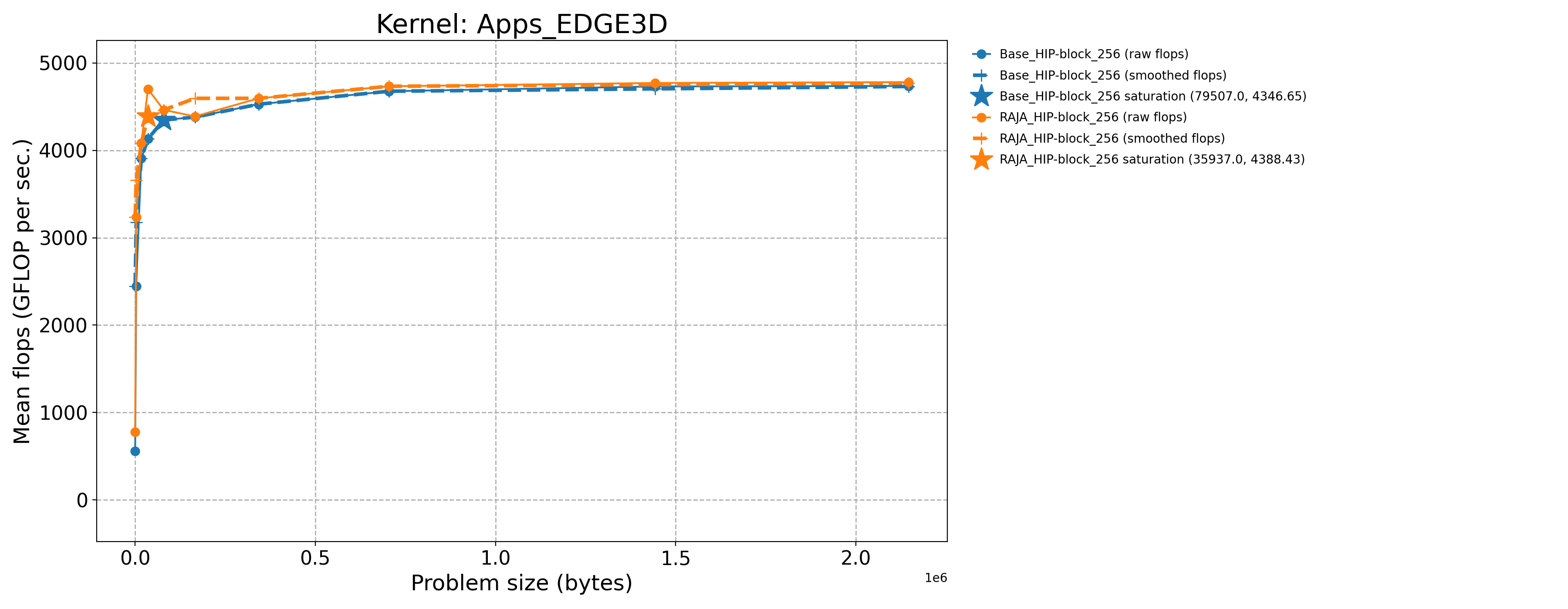
Apps_EDGE3D-Base_HIP-block_256 |
79507.0 |
4346.65 |
9.97035 |
Apps_EDGE3D-Base_Seq-default |
512.0 |
8.35478 |
0.0204122 |
Apps_EDGE3D-RAJA_HIP-block_256 |
35937.0 |
4701.17 |
10.8367 |
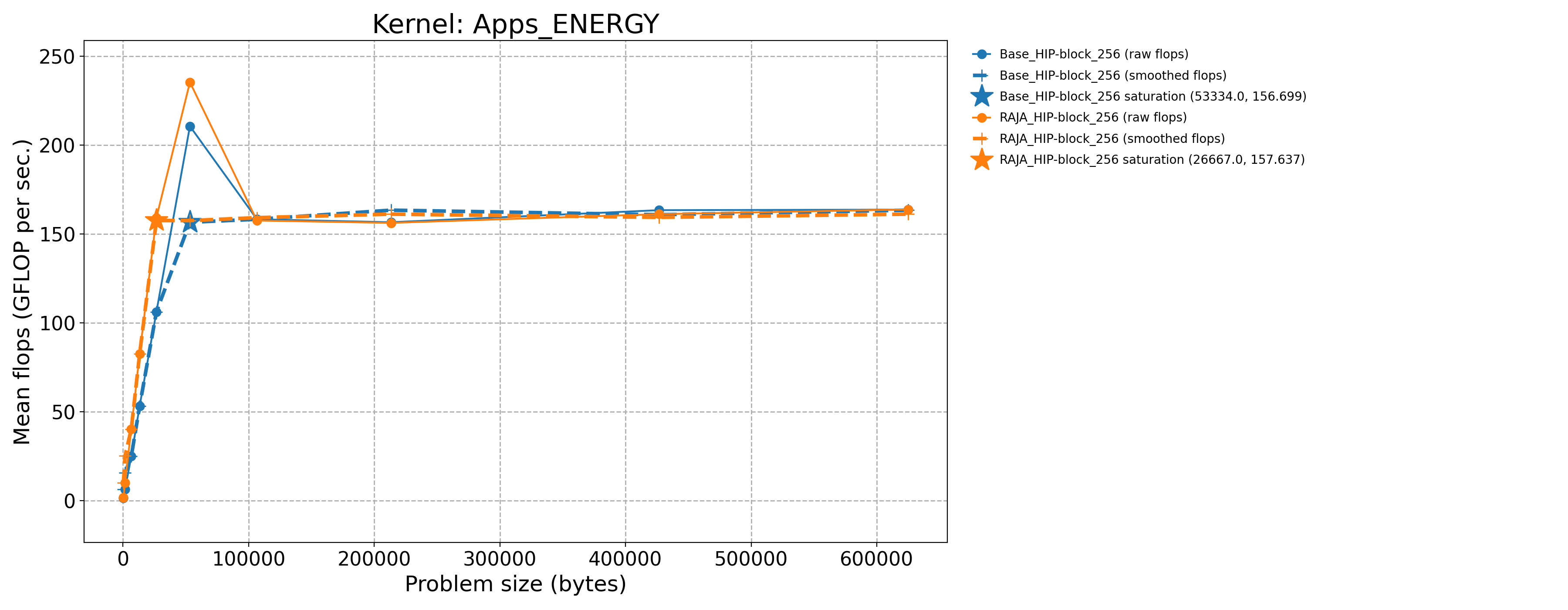
Apps_ENERGY-Base_HIP-block_256 |
53334.0 |
210.727 |
770.744 |
Apps_ENERGY-Base_Seq-default |
417.0 |
10.7796 |
39.4271 |
Apps_ENERGY-RAJA_HIP-block_256 |
26667.0 |
159.274 |
582.554 |
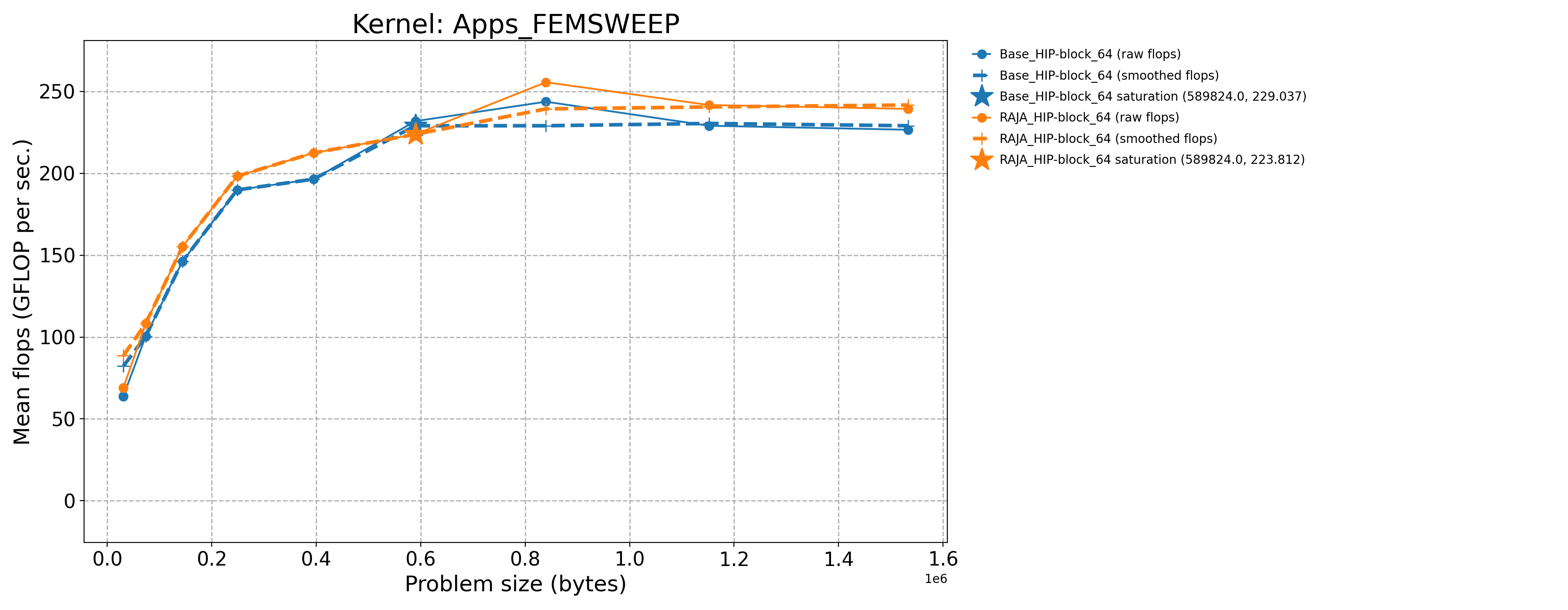
Apps_FEMSWEEP-Base_HIP-block_64 |
589824.0 |
231.835 |
44.4605 |
Apps_FEMSWEEP-Base_Seq-default |
31104.0 |
3.35637 |
0.602749 |
Apps_FEMSWEEP-RAJA_HIP-block_64 |
589824.0 |
223.812 |
42.9218 |
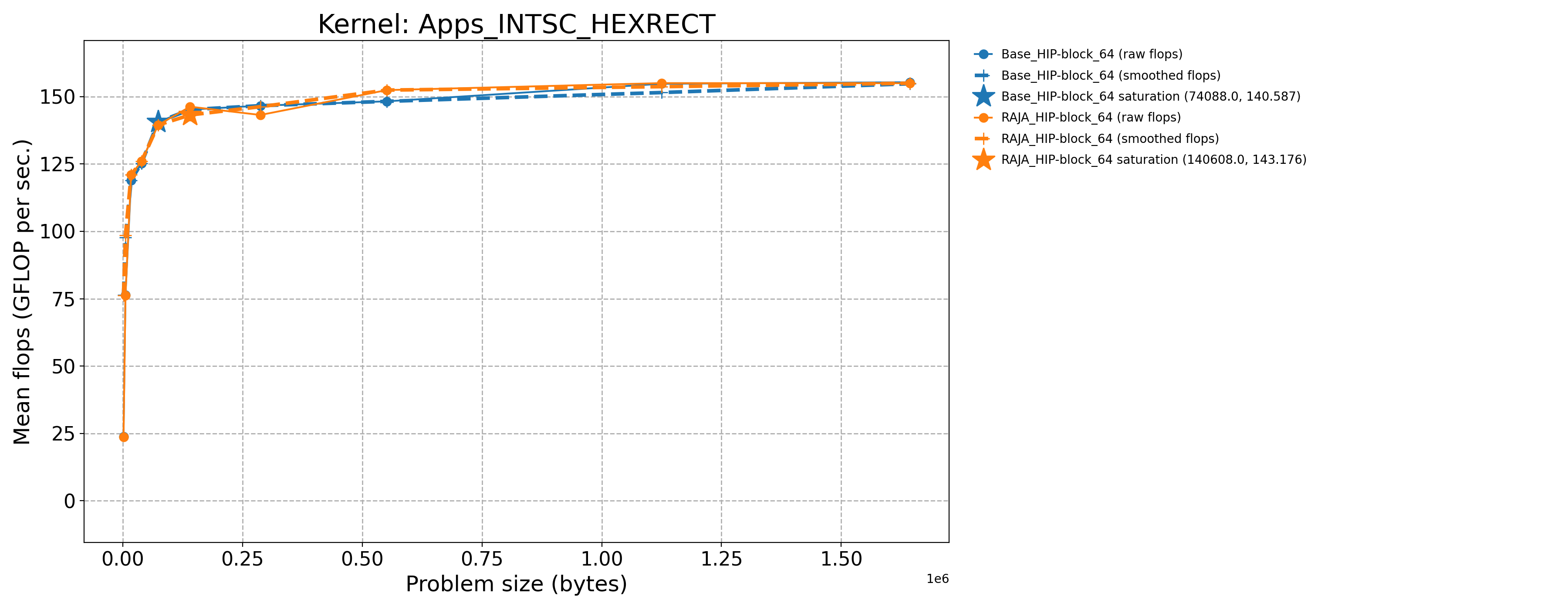
Apps_INTSC_HEXRECT-Base_HIP-block_64 |
74088.0 |
140.587 |
1.72573 |
Apps_INTSC_HEXRECT-Base_Seq-default |
1728.0 |
4.05739 |
0.0511849 |
Apps_INTSC_HEXRECT-RAJA_HIP-block_64 |
140608.0 |
146.252 |
1.79187 |
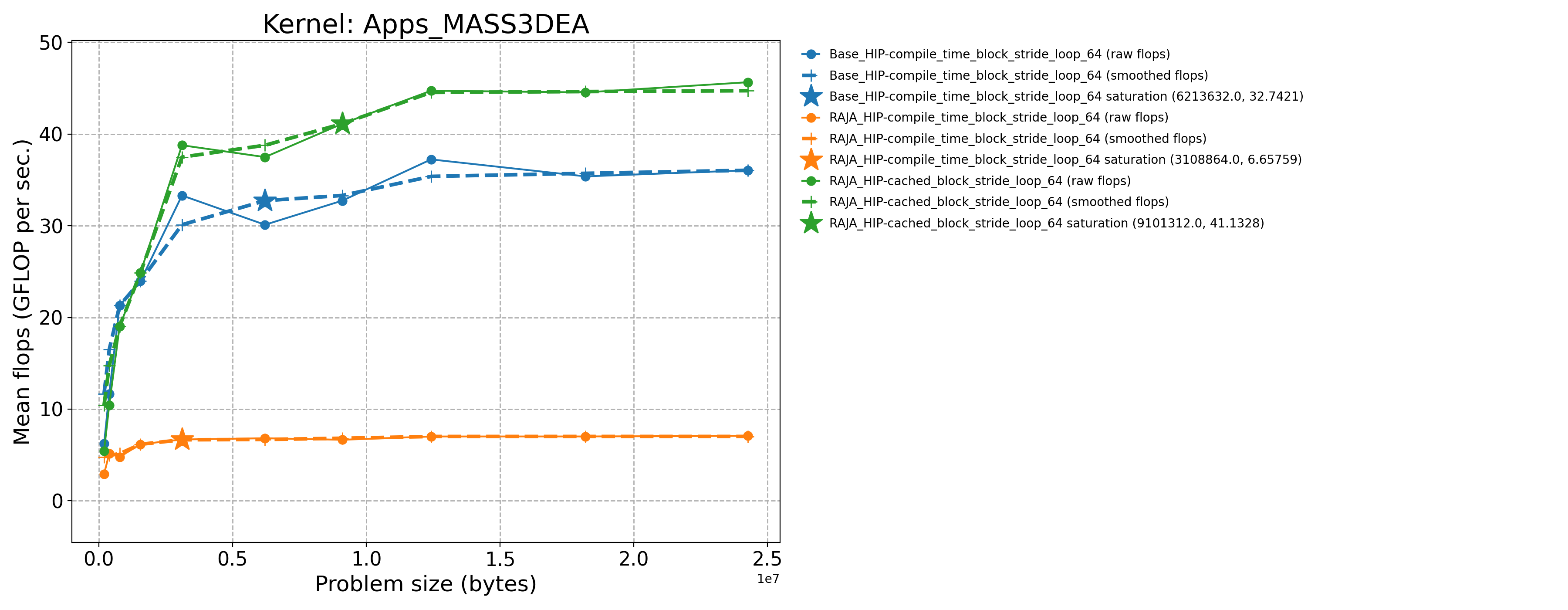
Apps_MASS3DEA-Base_HIP-compile_time_block_stride_loop_64 |
6213632.0 |
30.1164 |
33.0333 |
Apps_MASS3DEA-Base_Seq-default |
196608.0 |
0.0801476 |
0.0879186 |
Apps_MASS3DEA-RAJA_HIP-cached_block_stride_loop_64 |
9101312.0 |
41.1328 |
45.1167 |
Apps_MASS3DEA-RAJA_HIP-compile_time_block_stride_loop_64 |
3108864.0 |
6.68945 |
7.33737 |
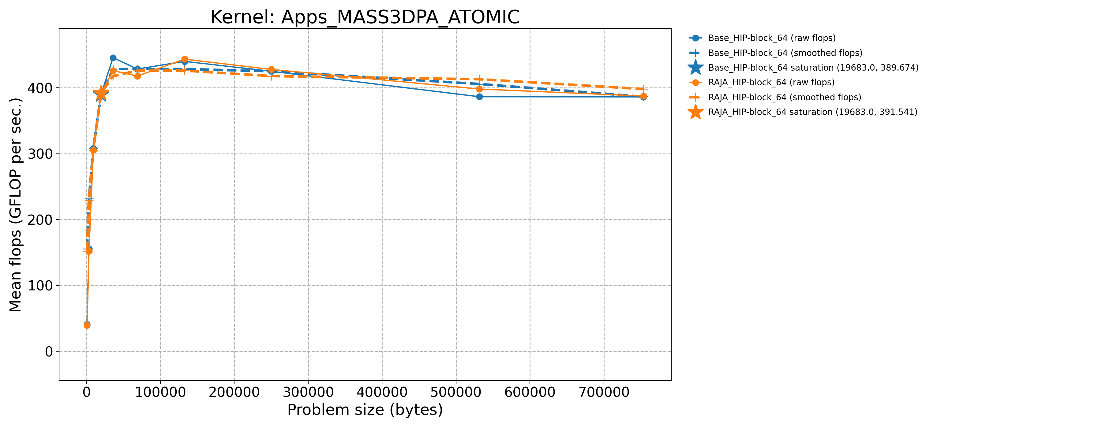
Apps_MASS3DPA_ATOMIC-Base_HIP-block_64 |
19683.0 |
389.674 |
183.315 |
Apps_MASS3DPA_ATOMIC-Base_Seq-default |
729.0 |
10.0932 |
5.04932 |
Apps_MASS3DPA_ATOMIC-RAJA_HIP-block_64 |
19683.0 |
391.541 |
184.193 |
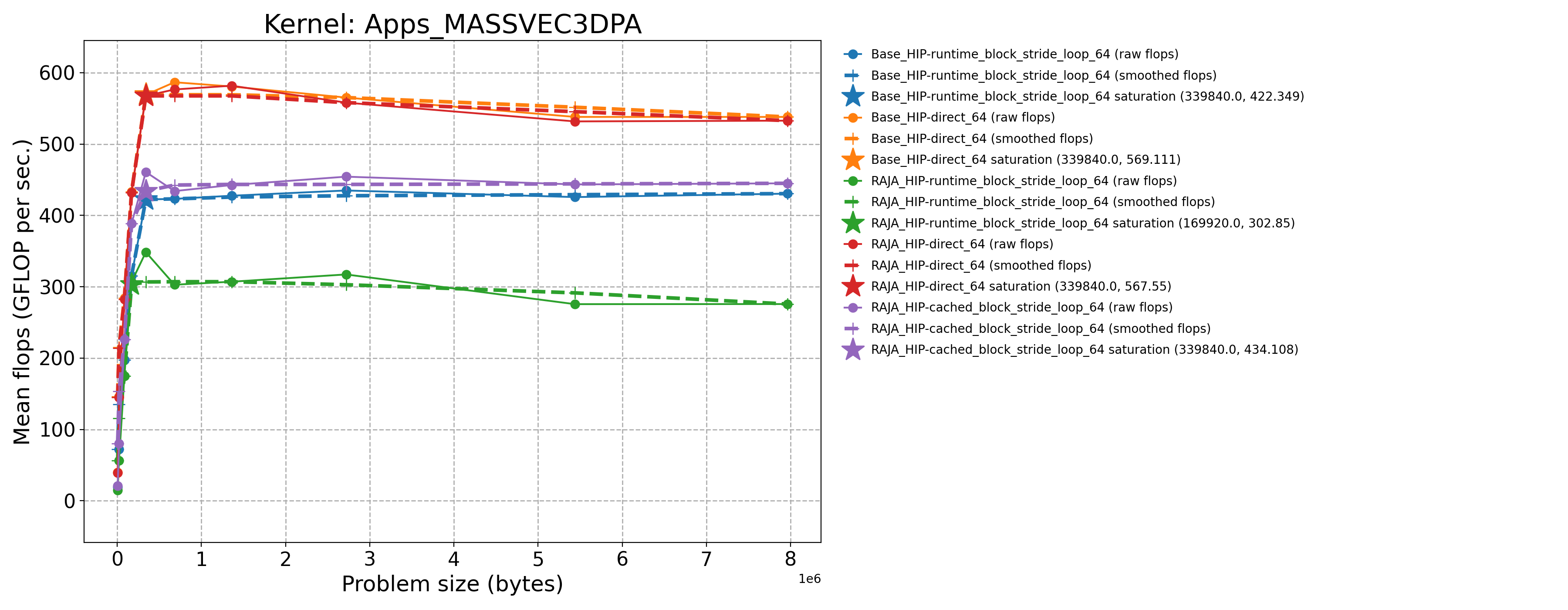
Apps_MASSVEC3DPA-Base_HIP-direct_64 |
339840.0 |
569.111 |
173.608 |
Apps_MASSVEC3DPA-Base_HIP-runtime_block_stride_loop_64 |
339840.0 |
422.349 |
128.838 |
Apps_MASSVEC3DPA-Base_Seq-default |
5376.0 |
10.7556 |
3.28712 |
Apps_MASSVEC3DPA-RAJA_HIP-cached_block_stride_loop_64 |
339840.0 |
460.798 |
140.567 |
Apps_MASSVEC3DPA-RAJA_HIP-direct_64 |
339840.0 |
567.55 |
173.132 |
Apps_MASSVEC3DPA-RAJA_HIP-runtime_block_stride_loop_64 |
169920.0 |
306.778 |
93.5856 |
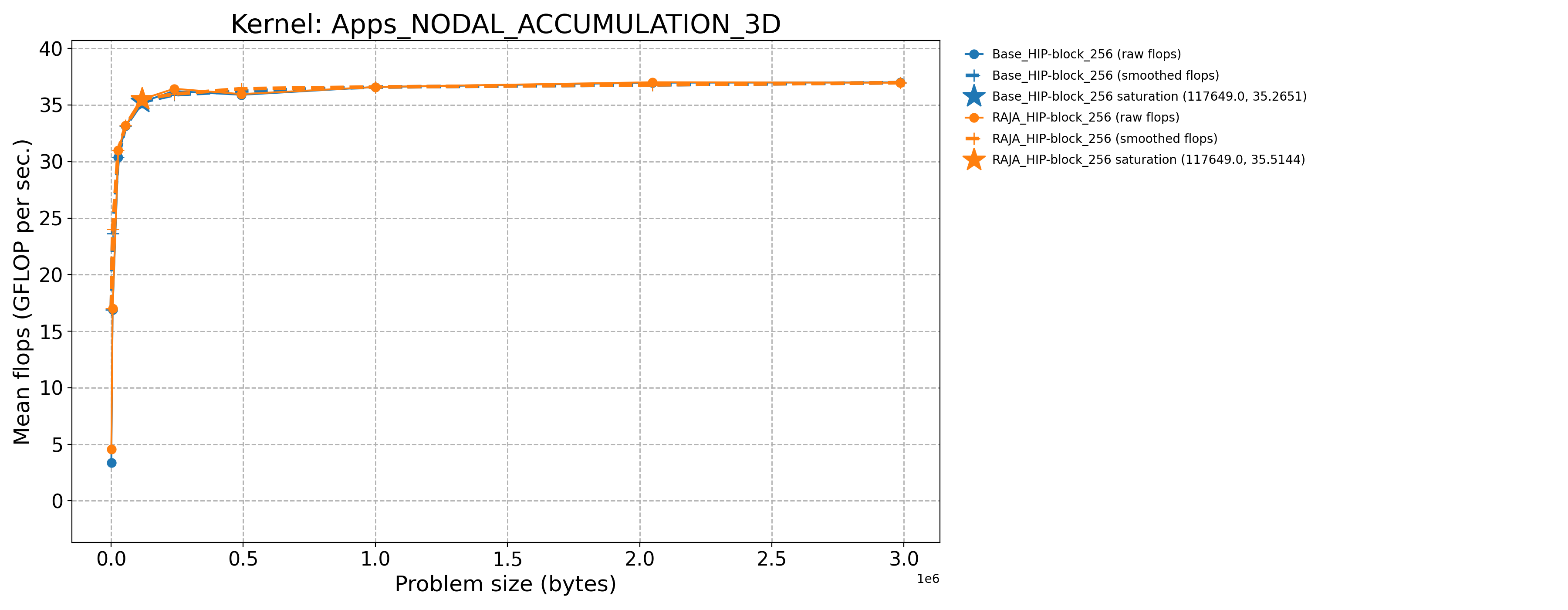
Apps_NODAL_ACCUMULATION_3D-Base_HIP-block_256 |
117649.0 |
35.2651 |
120.424 |
Apps_NODAL_ACCUMULATION_3D-Base_Seq-default |
1000.0 |
1.39273 |
5.37512 |
Apps_NODAL_ACCUMULATION_3D-RAJA_HIP-block_256 |
117649.0 |
35.5144 |
121.275 |
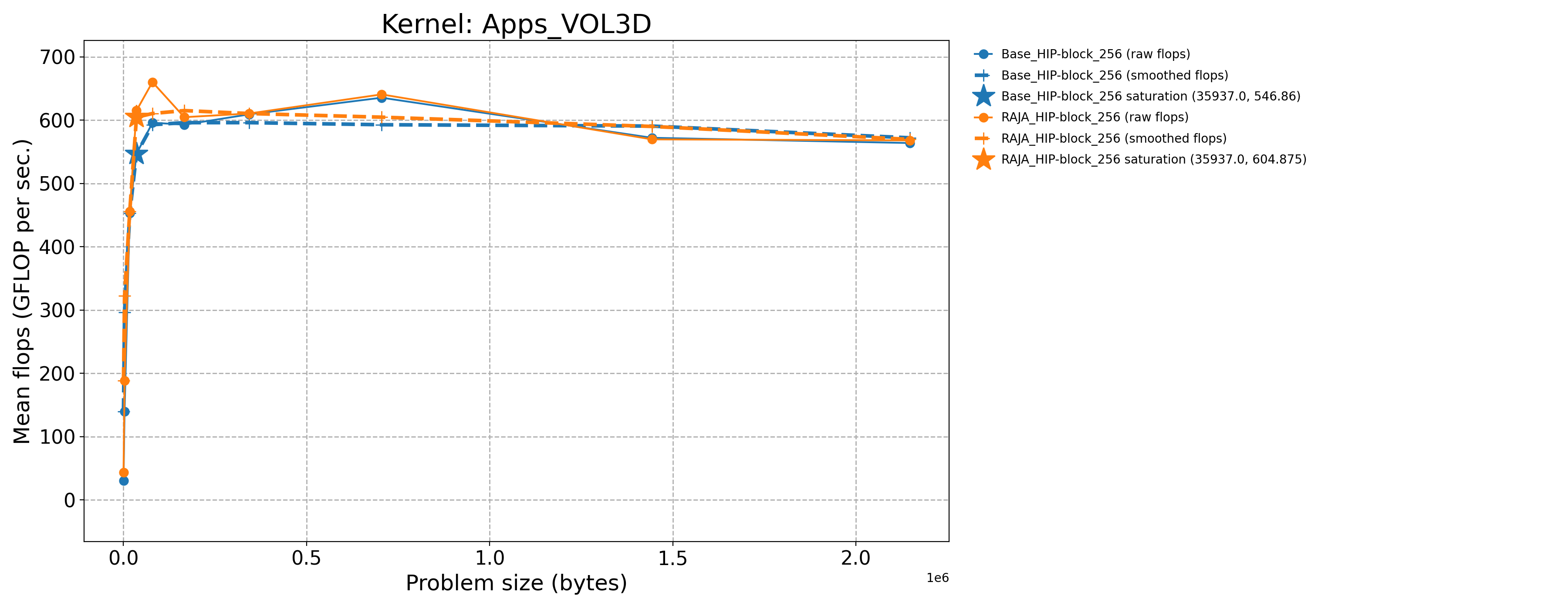
Apps_VOL3D-Base_HIP-block_256 |
35937.0 |
546.86 |
231.35 |
Apps_VOL3D-Base_Seq-default |
512.0 |
15.6567 |
7.02031 |
Apps_VOL3D-RAJA_HIP-block_256 |
35937.0 |
615.301 |
260.304 |
3.7.1.4. CPX mode (Priority 2)
The process for generating results for the Priority 2 kernels is essentially
the same as for the Priority 1 kernels just described. Note that two of the
kernels INDEXLIST_3LOOP and HALO_PACKING_FUSED do not perform any
floating point operations. They represent recurring computational patterns
in our application that are important rather than key numerical kernels.
Thus, the two kernels have zero GFLOP/sec rates. So, we consider the bandwidth
as the appropriate metric to consider.
Kernel |
Sat Problem Size |
Sat GFLOP/s |
Sat B/W (GiB per sec.) |
|---|---|---|---|
Apps_CONVECTION3DPA-Base_HIP-block_64 |
21951.0 |
358.542 |
198.044 |
Apps_CONVECTION3DPA-Base_Seq-default |
702.0 |
13.0552 |
7.24657 |
Apps_CONVECTION3DPA-RAJA_HIP-block_64 |
21951.0 |
350.353 |
193.521 |
Apps_DEL_DOT_VEC_2D-Base_HIP-block_256 |
32400.0 |
461.341 |
384.755 |
Apps_DEL_DOT_VEC_2D-Base_Seq-default |
841.0 |
8.22518 |
7.12761 |
Apps_DEL_DOT_VEC_2D-RAJA_HIP-block_256 |
32400.0 |
464.451 |
387.348 |
Apps_INTSC_HEXHEX-Base_HIP-block_64 |
216.0 |
3.12671 |
0.0674069 |
Apps_INTSC_HEXHEX-Base_Seq-default |
27.0 |
3.51739 |
0.0758293 |
Apps_INTSC_HEXHEX-RAJA_HIP-block_64 |
1000.0 |
5.84976 |
0.126111 |
Apps_LTIMES-Base_HIP-block_256 |
19392.0 |
109.457 |
152.356 |
Apps_LTIMES-Base_Seq-default |
1344.0 |
6.18006 |
8.69785 |
Apps_LTIMES-RAJA_HIP-kernel_256 |
19392.0 |
92.6917 |
129.02 |
Apps_LTIMES-RAJA_HIP-launch_256 |
19392.0 |
109.559 |
152.498 |
Apps_MASS3DPA-Base_HIP-block_25 |
101184.0 |
404.545 |
188.507 |
Apps_MASS3DPA-Base_Seq-default |
1600.0 |
11.1064 |
5.201 |
Apps_MASS3DPA-RAJA_HIP-block_25 |
101184.0 |
403.019 |
187.797 |
Apps_MATVEC_3D_STENCIL-Base_HIP-block_256 |
17576.0 |
172.721 |
443.39 |
Apps_MATVEC_3D_STENCIL-Base_Seq-default |
64.0 |
4.36214 |
15.3687 |
Apps_MATVEC_3D_STENCIL-RAJA_HIP-block_256 |
17576.0 |
183.707 |
471.59 |
Basic_INDEXLIST_3LOOP-Base_HIP-block_256 |
80000.0 |
0.0 |
146.085 |
Basic_INDEXLIST_3LOOP-Base_Seq-default |
80000.0 |
0.0 |
14.1788 |
Basic_INDEXLIST_3LOOP-RAJA_HIP-block_256 |
80000.0 |
0.0 |
143.168 |
Basic_MULTI_REDUCE-Base_HIP-atomic_direct_256 |
1599995.0 |
33.2328 |
495.21 |
Basic_MULTI_REDUCE-Base_HIP-atomic_occgs_256 |
1599995.0 |
33.4117 |
497.876 |
Basic_MULTI_REDUCE-Base_Seq-default |
3120.0 |
0.319886 |
4.78196 |
Basic_MULTI_REDUCE-RAJA_HIP-atomic_direct_256 |
799995.0 |
25.9727 |
387.028 |
Basic_MULTI_REDUCE-RAJA_HIP-atomic_occgs_256 |
1599995.0 |
33.0008 |
491.753 |
Basic_REDUCE_STRUCT-Base_HIP-blkatm_direct_256 |
50000.0 |
0.949965 |
7.07765 |
Basic_REDUCE_STRUCT-Base_HIP-blkatm_occgs_256 |
4687500.0 |
37.9404 |
282.678 |
Basic_REDUCE_STRUCT-Base_Seq-cascade |
3125.0 |
1.23615 |
9.20709 |
Basic_REDUCE_STRUCT-Base_Seq-default |
3125.0 |
2.28624 |
17.0284 |
Basic_REDUCE_STRUCT-Base_Seq-kahan |
3125.0 |
0.607103 |
4.52183 |
Basic_REDUCE_STRUCT-RAJA_HIP-blkatm_direct_256 |
800000.0 |
9.13983 |
68.097 |
Basic_REDUCE_STRUCT-RAJA_HIP-blkatm_occgs_256 |
1600000.0 |
48.9732 |
364.879 |
Basic_REDUCE_STRUCT-RAJA_HIP-blkdev_direct_256 |
800000.0 |
7.94678 |
59.208 |
Basic_REDUCE_STRUCT-RAJA_HIP-blkdev_direct_new_256 |
800000.0 |
5.64748 |
42.077 |
Basic_REDUCE_STRUCT-RAJA_HIP-blkdev_occgs_256 |
1600000.0 |
43.8298 |
326.557 |
Basic_REDUCE_STRUCT-RAJA_HIP-blkdev_occgs_new_256 |
3200000.0 |
47.4026 |
353.177 |
Comm_HALO_PACKING_FUSED-Base_HIP-direct_1024 |
42875.0 |
0.0 |
35.5465 |
Comm_HALO_PACKING_FUSED-Base_Seq-direct |
42875.0 |
0.0 |
34.2866 |
Comm_HALO_PACKING_FUSED-RAJA_HIP-direct_1024 |
42875.0 |
0.0 |
28.3649 |
Comm_HALO_PACKING_FUSED-RAJA_HIP-funcptr_1024 |
42875.0 |
0.0 |
30.9433 |
Comm_HALO_PACKING_FUSED-RAJA_HIP-virtfunc_1024 |
42875.0 |
0.0 |
29.0926 |
The baseline data files for Priority 2 kernels run on this MI300A architecture in
CPX mode are in this repo in the directory ./docs/13_rajaperf/baseline_data/RPBenchmark_MI300A_tier1-CPX.
3.7.1.5. AMD MI300A throughput plots (Priority 1)
The following table contains throughput plots for each kernel run as described above on the MI300A architecture in SPX mode and CPX mode. Each plot has multiple curves with GFLOP/sec (compute rate) plotted as a function of problem size (allocated bytes). The left column shows SPX mode. The right column shows CPX mode. The legend in each plot indicates the curves shown. Each plot includes:
Throughput curves for Base and RAJA variant(s) of the kernel (solid line segments connecting the dots, where the dots are actual GFLOP rates determined from the kernel being run at a given problem size).
Smoothed versions of the throughput curves (dashed lines), which are constructed from the dots.
Stars that indicate approximate saturation points based on the smoothed curves and computed using simple heuristics. The legend contains the (x, y) values for the saturation points.
Most plots contain two variants, with the non-RAJA variant in blue and RAJA variant in orange. In these cases, the throughput and saturation are close, which indicates that the RAJA variants perform as well as the non-RAJA variants that are written directly in HIP with no RAJA abstractions. Two kernels (MASS3DEA, MASSVEC3DPA) contain additional curves that show more variants. These additional curves are included to show how kernel execution choices, RAJA execution policies specifically, can have a significant impact on performance.
Priority 1 Kernels: MI300A Node Throughput (SPX Mode) |
Priority 1 Kernels: MI300A Node Throughput (CPX Mode) |
|
|
|
|
|
|
|
|
|
|
|
|
|
|
|
|
|
|
|
|
3.7.2. NVIDIA H100 throughput results (Priority 1 kernels)
For the H100 architecture, we present throughput results, where we run with
4 MPI ranks on a node – one for each H100 GPU. We run each Priority 1
kernel over a sequence of problem sizes such that the saturation point is
evident on its associated throughput curve.
We choose the smallest problem to use ~50,000 bytes of allocated memory and the largest problem to use ~150MB of allocated memory, which is about 3 times the L2 cache size on the H100 GPU. The L2 cache is 50 MB (50 * 1024 * 1024 = 52428800 bytes).
Note that for two of the kernels FEMSWEEP and MASS3DEA, we ran a
different problem size range because these kernels don’t clearly saturate.
For them, we chose the smallest problem to use ~1.6MB of allocated memory
and the largest problem to use ~300MB memory, which is about 6 times the
L2 cache size.
After building the code as described in H100 architecture, we
run the Priority 1 kernels as follows:
$ pwd
path/to/RAJAPerf
$ cd build_lc_toss4-mvapich2-2.3.7-nvcc-12.9.1-90-gcc-10.3.1
$ ./run_tier_h100.sh tier1
This generates a directory named RPBenchmark_H100_tier1, which contains
the results files for each kernel run over its range of problem sizes.
Then, we process the data for reporting the results here in a concise form by running a Python script we provide:
$ pwd
path/to/RAJAPerf
$ python3 path/to/process_data.py --root-dir path/to/build_lc_toss4-mvapich2-2.3.7-nvcc-12.9.1-90-gcc-10.3.1/RPBenchmark_H100_tier1 --output-dir path/to/build_lc_toss4-mvapich2-2.3.7-nvcc-12.9.1-90-gcc-10.3.1/RPBenchmark_H100_tier1/Output
This generates throughput curve files for Base_HIP and RAJA_HIP
variants of each kernel and summarizes the FOM (described in
Figure of Merit) in a CSV file. These files will be located in the
directory specified by via the --output-dir option above. We include
the files generated by the process_data.py script in this repo in the
directory ./docs/13_rajaperf/baseline_data/RPBenchmark_H100_tier1.
Kernel |
Sat Problem Size |
Sat GFLOP/s |
Sat B/W (GiB per sec.) |
|---|---|---|---|
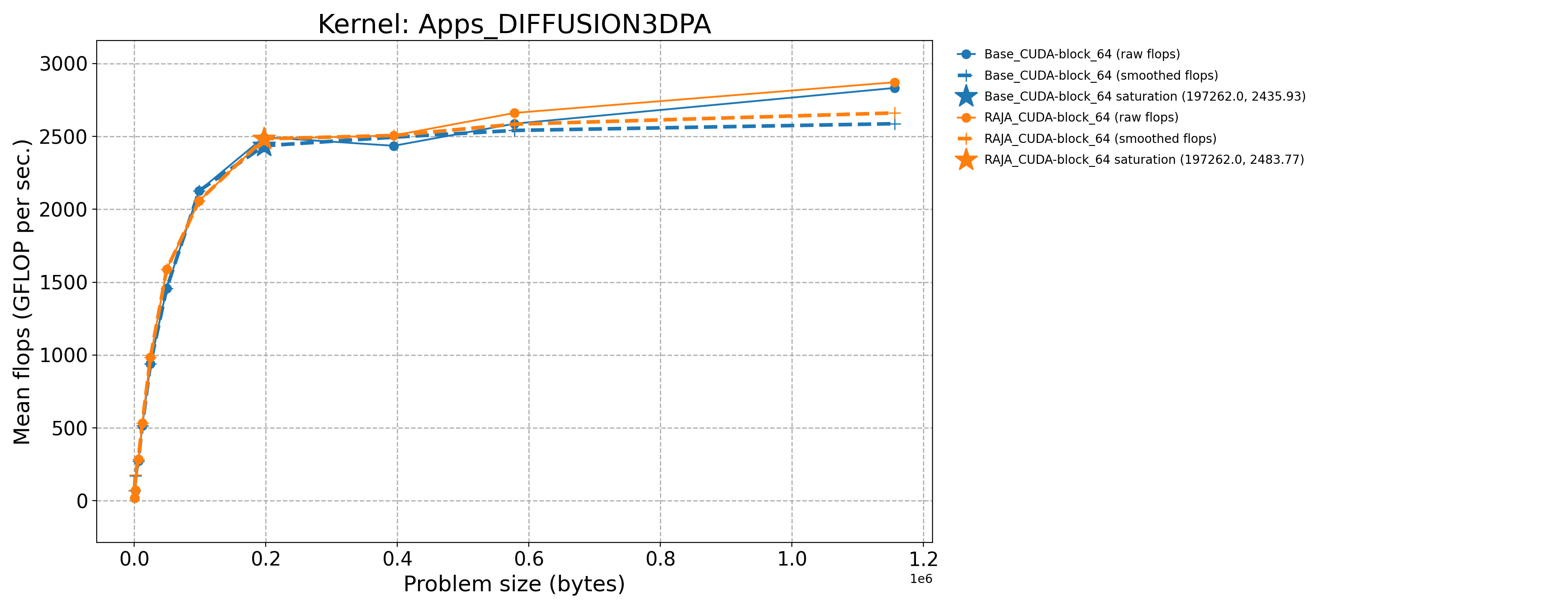
Apps_DIFFUSION3DPA-Base_CUDA-block_64 |
197262.0 |
2495.05 |
1662.67 |
Apps_DIFFUSION3DPA-Base_Seq-default |
405.0 |
13.1459 |
8.79032 |
Apps_DIFFUSION3DPA-RAJA_CUDA-block_64 |
197262.0 |
2483.77 |
1655.15 |
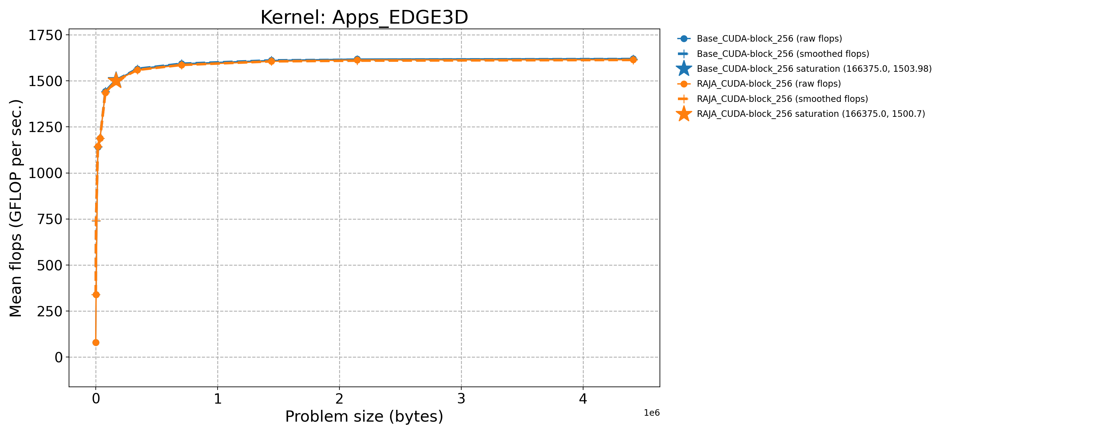
Apps_EDGE3D-Base_CUDA-block_256 |
166375.0 |
1503.98 |
3.43745 |
Apps_EDGE3D-Base_Seq-default |
512.0 |
9.38302 |
0.0229243 |
Apps_EDGE3D-RAJA_CUDA-block_256 |
166375.0 |
1500.7 |
3.42995 |
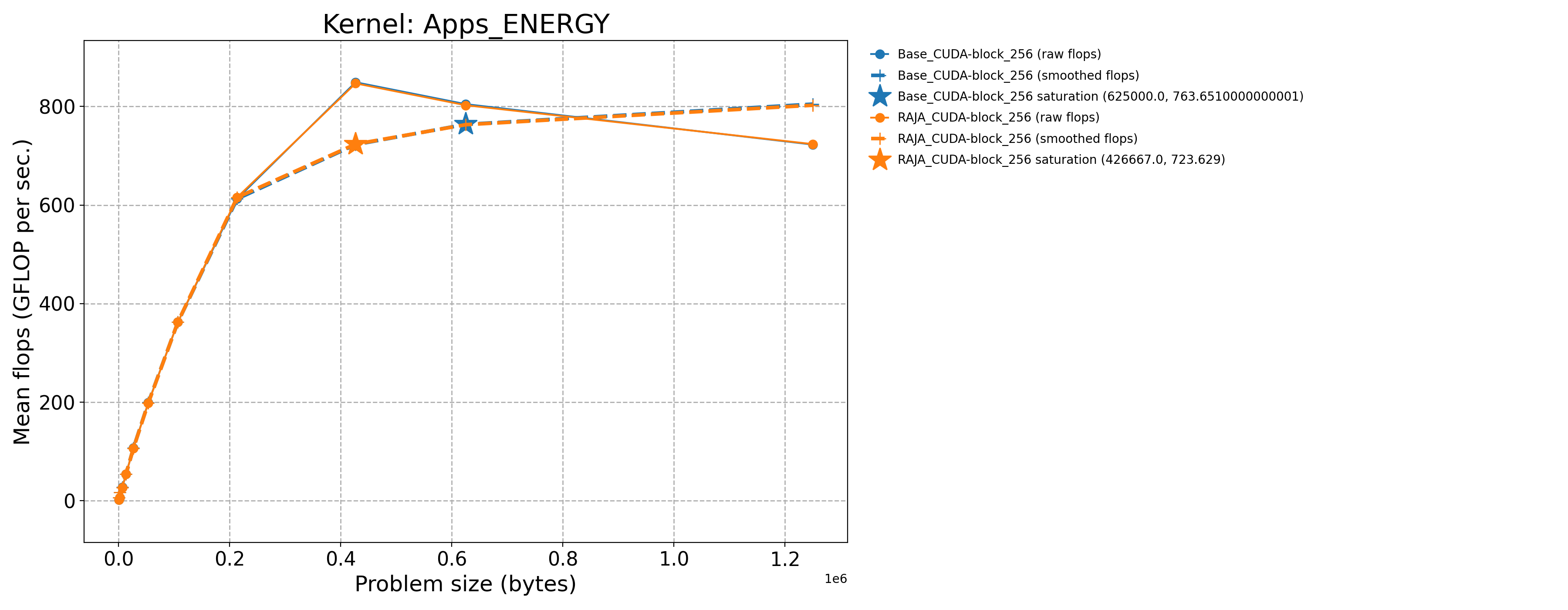
Apps_ENERGY-Base_CUDA-block_256 |
625000.0 |
804.683 |
2943.18 |
Apps_ENERGY-Base_Seq-default |
417.0 |
13.341 |
48.7956 |
Apps_ENERGY-RAJA_CUDA-block_256 |
426667.0 |
846.742 |
3097.01 |
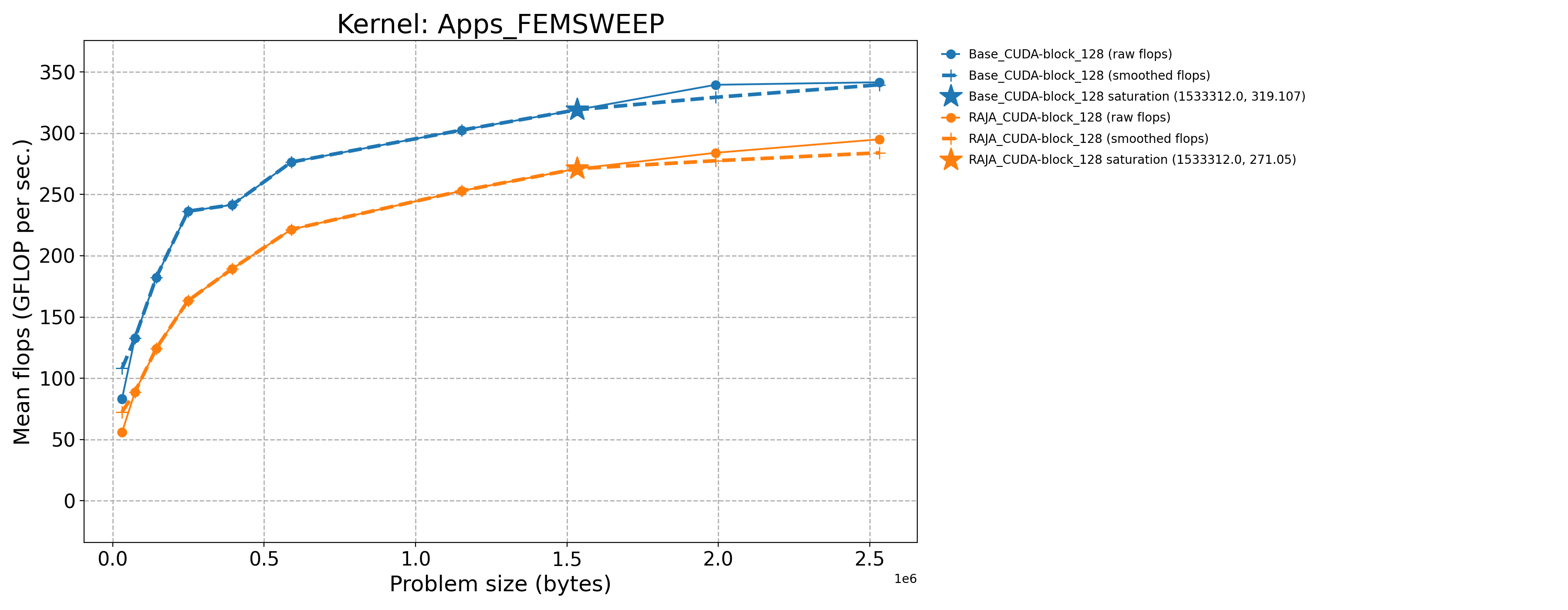
Apps_FEMSWEEP-Base_CUDA-block_128 |
1533312.0 |
319.107 |
61.8105 |
Apps_FEMSWEEP-Base_Seq-default |
31104.0 |
3.31578 |
0.595459 |
Apps_FEMSWEEP-RAJA_CUDA-block_128 |
1533312.0 |
271.05 |
52.502 |
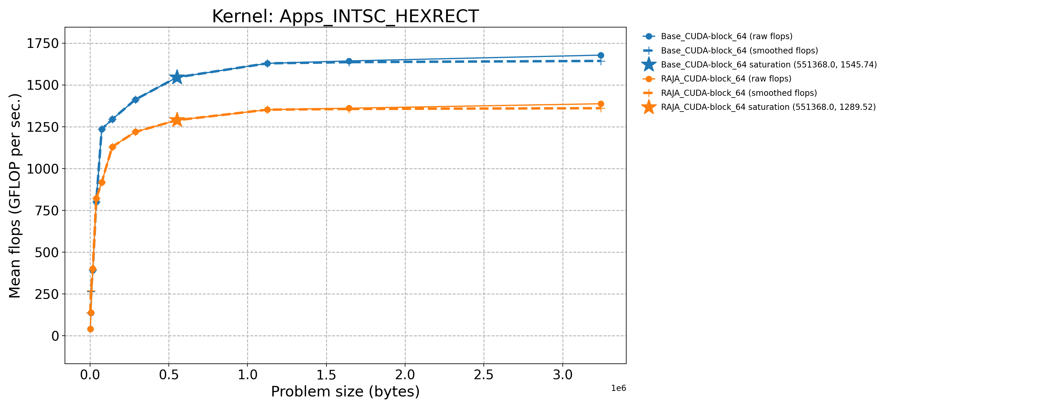
Apps_INTSC_HEXRECT-Base_CUDA-block_64 |
551368.0 |
1545.74 |
18.8845 |
Apps_INTSC_HEXRECT-Base_Seq-default |
1728.0 |
4.08557 |
0.0515405 |
Apps_INTSC_HEXRECT-RAJA_CUDA-block_64 |
551368.0 |
1289.52 |
15.7543 |
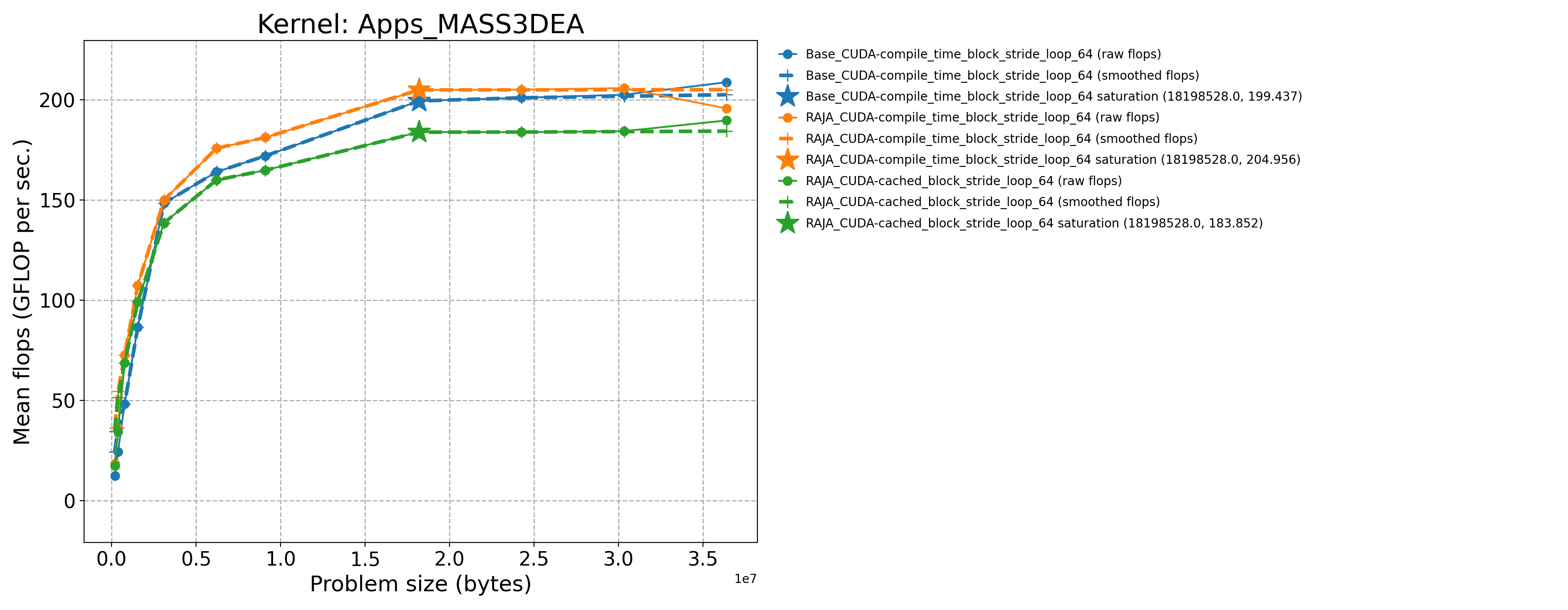
Apps_MASS3DEA-Base_CUDA-compile_time_block_stride_loop_64 |
18198528.0 |
199.437 |
218.752 |
Apps_MASS3DEA-Base_Seq-default |
196608.0 |
0.172475 |
0.189198 |
Apps_MASS3DEA-RAJA_CUDA-cached_block_stride_loop_64 |
18198528.0 |
183.938 |
201.752 |
Apps_MASS3DEA-RAJA_CUDA-compile_time_block_stride_loop_64 |
18198528.0 |
204.956 |
224.806 |
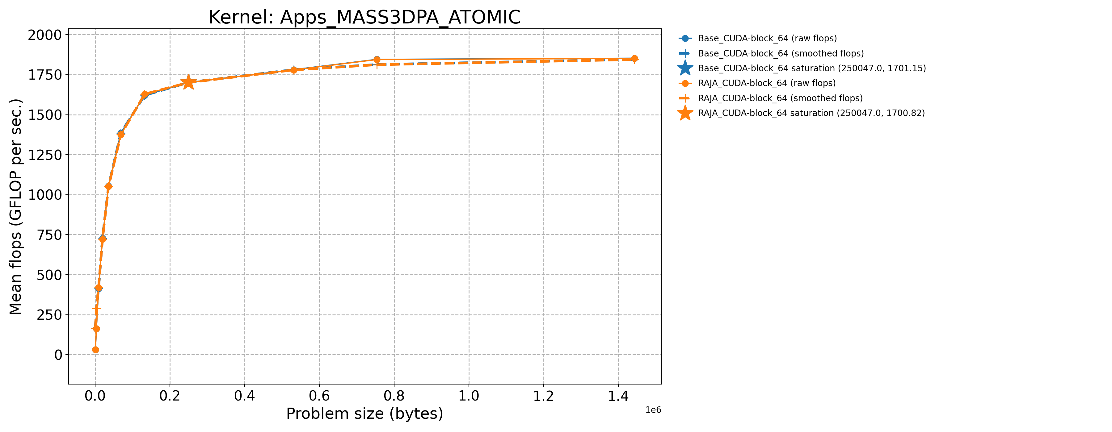
Apps_MASS3DPA_ATOMIC-Base_CUDA-block_64 |
250047.0 |
1701.15 |
788.718 |
Apps_MASS3DPA_ATOMIC-Base_Seq-default |
729.0 |
11.2564 |
5.63123 |
Apps_MASS3DPA_ATOMIC-RAJA_CUDA-block_64 |
250047.0 |
1700.82 |
788.566 |
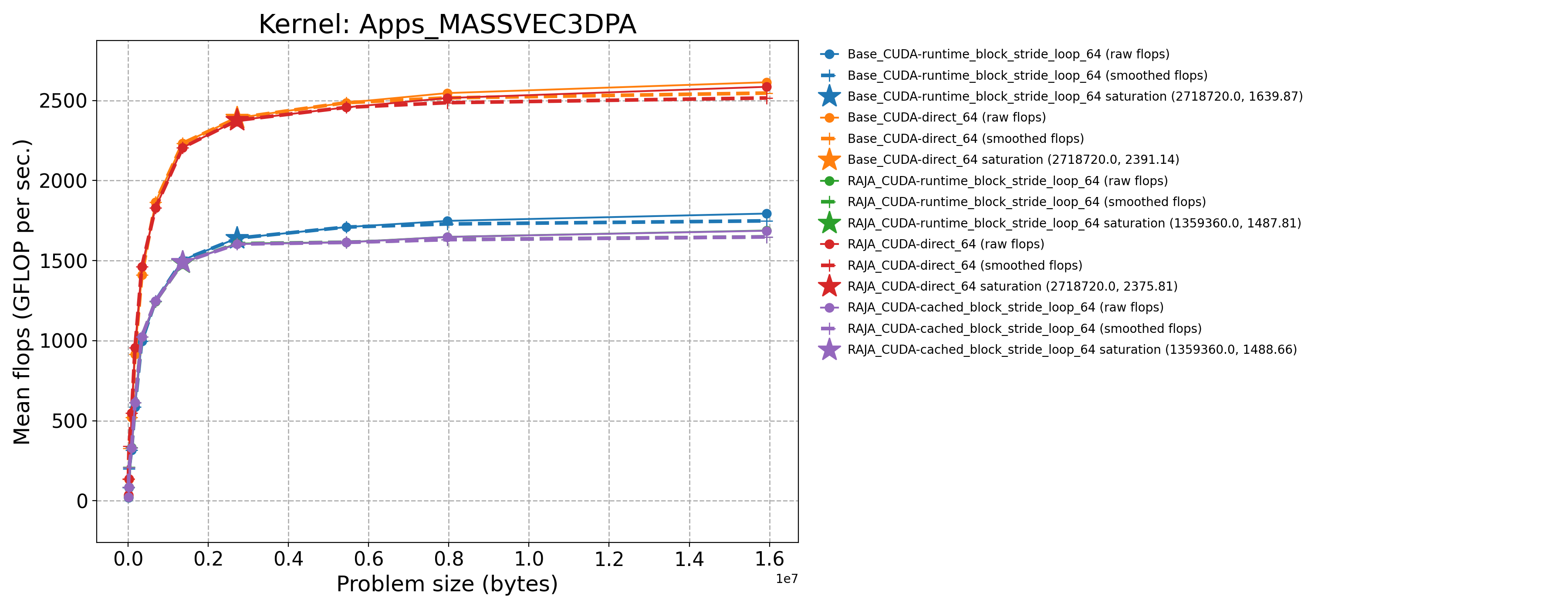
Apps_MASSVEC3DPA-Base_CUDA-direct_64 |
2718720.0 |
2391.14 |
729.4 |
Apps_MASSVEC3DPA-Base_CUDA-runtime_block_stride_loop_64 |
2718720.0 |
1639.87 |
500.232 |
Apps_MASSVEC3DPA-Base_Seq-default |
5376.0 |
12.7342 |
3.89184 |
Apps_MASSVEC3DPA-RAJA_CUDA-cached_block_stride_loop_64 |
1359360.0 |
1488.66 |
454.106 |
Apps_MASSVEC3DPA-RAJA_CUDA-direct_64 |
2718720.0 |
2375.81 |
724.725 |
Apps_MASSVEC3DPA-RAJA_CUDA-runtime_block_stride_loop_64 |
1359360.0 |
1487.81 |
453.847 |
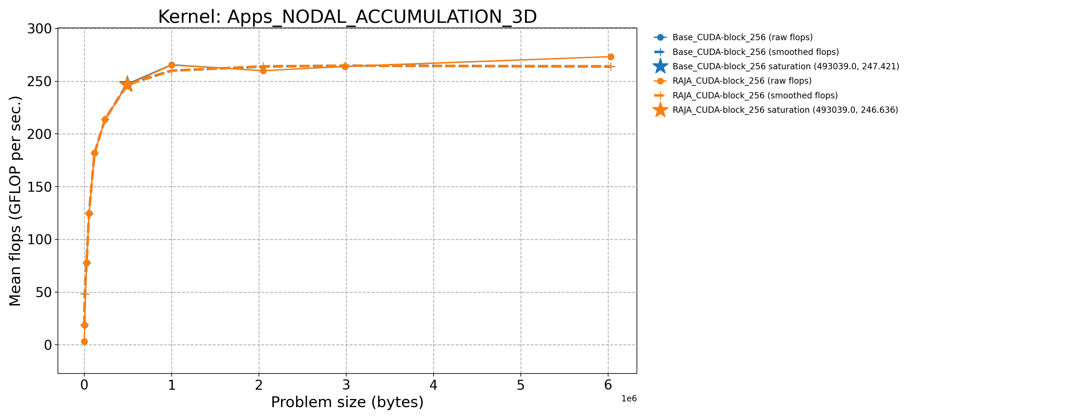
Apps_NODAL_ACCUMULATION_3D-Base_CUDA-block_256 |
493039.0 |
247.421 |
835.056 |
Apps_NODAL_ACCUMULATION_3D-Base_Seq-default |
1000.0 |
4.25353 |
16.4161 |
Apps_NODAL_ACCUMULATION_3D-RAJA_CUDA-block_256 |
493039.0 |
246.636 |
832.406 |
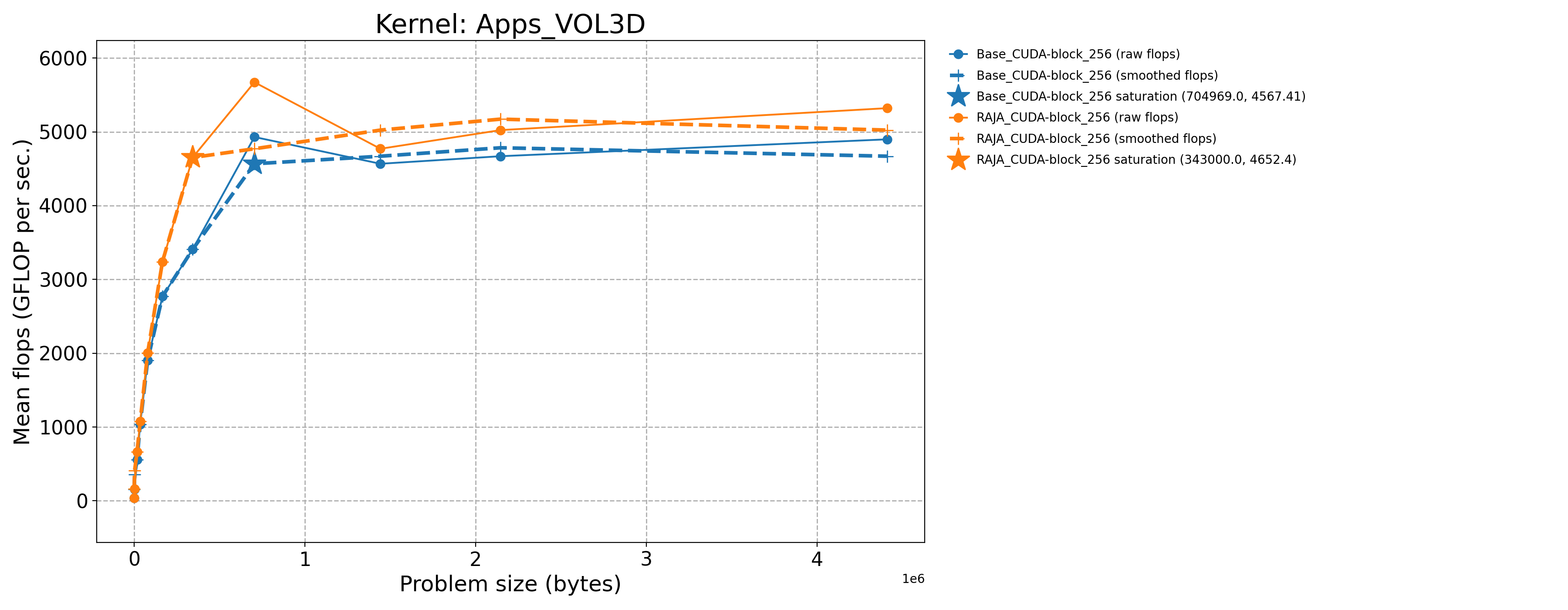
Apps_VOL3D-Base_CUDA-block_256 |
704969.0 |
4930.32 |
2057.77 |
Apps_VOL3D-Base_Seq-default |
512.0 |
10.589 |
4.748 |
Apps_VOL3D-RAJA_CUDA-block_256 |
343000.0 |
4652.4 |
1946.07 |
3.7.2.1. H100 (Priority 2)
The process for generating results for the Priority 2 kernels is essentially
the same as for the Priority 1 kernels just described. Note that two of the
kernels INDEXLIST_3LOOP and HALO_PACKING_FUSED do not perform any
floating point operations. They represent recurring computational patterns
in our application that are important rather than key numerical kernels.
Thus, the two kernels have zero GFLOP/sec rates. So, we consider the bandwidth
as the appropriate metric to consider.
Kernel |
Sat Problem Size |
Sat GFLOP/s |
Sat B/W (GiB per sec.) |
|---|---|---|---|
Apps_CONVECTION3DPA-Base_CUDA-block_64 |
351216.0 |
2353.16 |
1299.59 |
Apps_CONVECTION3DPA-Base_Seq-default |
702.0 |
16.2141 |
8.99998 |
Apps_CONVECTION3DPA-RAJA_CUDA-block_64 |
351216.0 |
2343.2 |
1294.09 |
Apps_DEL_DOT_VEC_2D-Base_CUDA-block_256 |
264196.0 |
2752.57 |
2284.61 |
Apps_DEL_DOT_VEC_2D-Base_Seq-default |
841.0 |
10.3907 |
9.00417 |
Apps_DEL_DOT_VEC_2D-RAJA_CUDA-block_256 |
264196.0 |
2752.84 |
2284.84 |
Apps_INTSC_HEXHEX-Base_CUDA-block_64 |
1728.0 |
1055.5 |
22.7549 |
Apps_INTSC_HEXHEX-Base_Seq-default |
27.0 |
4.59175 |
0.0989909 |
Apps_INTSC_HEXHEX-RAJA_CUDA-block_64 |
1728.0 |
1054.95 |
22.7431 |
Apps_LTIMES-Base_CUDA-block_256 |
309696.0 |
642.991 |
894.303 |
Apps_LTIMES-Base_Seq-default |
1344.0 |
5.10678 |
7.18731 |
Apps_LTIMES-RAJA_CUDA-kernel_256 |
309696.0 |
636.478 |
885.243 |
Apps_LTIMES-RAJA_CUDA-launch_256 |
309696.0 |
657.487 |
914.464 |
Apps_MASS3DPA-Base_CUDA-block_25 |
809536.0 |
3074.41 |
1432.49 |
Apps_MASS3DPA-Base_Seq-default |
1600.0 |
14.0527 |
6.5807 |
Apps_MASS3DPA-RAJA_CUDA-block_25 |
809536.0 |
3060.07 |
1425.82 |
Apps_MATVEC_3D_STENCIL-Base_CUDA-block_256 |
79507.0 |
774.039 |
1932.98 |
Apps_MATVEC_3D_STENCIL-Base_Seq-default |
64.0 |
5.01708 |
17.6762 |
Apps_MATVEC_3D_STENCIL-RAJA_CUDA-block_256 |
157464.0 |
939.463 |
2325.58 |
Basic_INDEXLIST_3LOOP-Base_CUDA-block_256 |
80000.0 |
0.0 |
185.245 |
Basic_INDEXLIST_3LOOP-Base_Seq-default |
80000.0 |
0.0 |
6.21439 |
Basic_INDEXLIST_3LOOP-RAJA_CUDA-block_256 |
80000.0 |
0.0 |
182.04 |
Basic_MULTI_REDUCE-Base_CUDA-atomic_direct_256 |
18749995.0 |
16.7769 |
249.995 |
Basic_MULTI_REDUCE-Base_CUDA-atomic_occgs_256 |
15624995.0 |
13.2005 |
196.703 |
Basic_MULTI_REDUCE-Base_Seq-default |
99995.0 |
0.467413 |
6.96569 |
Basic_MULTI_REDUCE-RAJA_CUDA-atomic_direct_256 |
18749995.0 |
16.721 |
249.162 |
Basic_MULTI_REDUCE-RAJA_CUDA-atomic_occgs_256 |
15624995.0 |
12.9928 |
193.607 |
Basic_REDUCE_STRUCT-Base_CUDA-blkatm_direct_256 |
18750000.0 |
43.1103 |
321.197 |
Basic_REDUCE_STRUCT-Base_CUDA-blkatm_occgs_256 |
18750000.0 |
47.2183 |
351.804 |
Basic_REDUCE_STRUCT-Base_Seq-cascade |
100000.0 |
0.903853 |
6.73416 |
Basic_REDUCE_STRUCT-Base_Seq-default |
100000.0 |
1.88462 |
14.0414 |
Basic_REDUCE_STRUCT-Base_Seq-kahan |
100000.0 |
0.945023 |
7.0409 |
Basic_REDUCE_STRUCT-RAJA_CUDA-blkatm_direct_256 |
15625000.0 |
26.846 |
200.018 |
Basic_REDUCE_STRUCT-RAJA_CUDA-blkatm_occgs_256 |
15625000.0 |
26.1101 |
194.536 |
Basic_REDUCE_STRUCT-RAJA_CUDA-blkdev_direct_256 |
800000.0 |
24.3351 |
181.31 |
Basic_REDUCE_STRUCT-RAJA_CUDA-blkdev_direct_new_256 |
4687500.0 |
33.959 |
253.014 |
Basic_REDUCE_STRUCT-RAJA_CUDA-blkdev_occgs_256 |
12500000.0 |
272.671 |
2031.56 |
Basic_REDUCE_STRUCT-RAJA_CUDA-blkdev_occgs_new_256 |
12500000.0 |
263.766 |
1965.21 |
Comm_HALO_PACKING_FUSED-Base_CUDA-direct_1024 |
42875.0 |
0.0 |
27.8679 |
Comm_HALO_PACKING_FUSED-Base_Seq-direct |
42875.0 |
0.0 |
37.5249 |
Comm_HALO_PACKING_FUSED-RAJA_CUDA-direct_1024 |
42875.0 |
0.0 |
24.3736 |
Comm_HALO_PACKING_FUSED-RAJA_CUDA-funcptr_1024 |
42875.0 |
0.0 |
22.4841 |
Comm_HALO_PACKING_FUSED-RAJA_CUDA-virtfunc_1024 |
42875.0 |
0.0 |
22.6106 |
The baseline data files for Priority 2 kernels run on the H100 architecture
are in this repo in the directory ./docs/13_rajaperf/baseline_data/RPBenchmark_H100_tier2-SPX.
3.7.2.2. NVIDIA H100 throughput plots (Priority 1)
The following table contains throughput plots for each kernel run as described above for the H100 architecture. Each plot has multiple curves where GFLOP/sec (compute rate) is plotted as a function of problem size (allocated bytes). The legend in each plot indicates the curves shown. Each plot includes:
Throughput curves for Base and RAJA variant(s) of the kernel (solid line segments connecting the dots, where the dots are actual GFLOP rates determined from the kernel being run at a given problem size).
Smoothed versions of the throughput curves (dashed lines), which are constructed from the dots.
Stars that indicate approximate saturation points based on the smoothed curves and computed using simple heuristics. The legend contains the (x, y) values for the saturation points.
Most plots contain two variants, with the non-RAJA variant in blue and RAJA variant in orange. In these cases, the throughput and saturation are close, which indicates that the RAJA variants perform as well as the non-RAJA variants that are written directly in CUDA with no RAJA abstractions. Two kernels (MASS3DEA, MASSVEC3DPA) contain additional curves that show more variants. These additional curves were included to show how kernel execution choices, RAJA execution policies specifically, can have a noticeable impact on performance.
Priority 1 Kernels H100 Node Throughput |
|
|
|
|
|
|
|
|
|
|
3.8. Memory Usage
For the RAJA Performance Suite Benchmark, we run each kernel over a sequence of problem sizes to generate a throughput curve and, based on that, estimate a saturation point. The memory usage for each entry in the sequence is roughly the same for each kernel. However, there is no significant meaning to take away from this since the memory usage of kernels like those in the Suite will be determined by the application context in which they are used.
3.9. Strong Scaling on El Capitan
The RAJA Performance Suite is primarily a single-node and compiler assessment tool. Thus, strong scaling is not part of the benchmark.
3.10. Weak Scaling on El Capitan
The RAJA Performance Suite is primarily a single-node and compiler assessment tool. Thus, weak scaling is not part of the benchmark.
3.11. References
The GitHub repositories are the primary references for RAJA and the RAJA Performance Suite:
Other helpful references include:
Olga Pearce, Jason Burmark, Rich Hornung, Befikir Bogale, Ian Lumsden, Michael McKinsey, Dewi Yokelson, David Boehme, Stephanie Brink, Michela Taufer, Tom Scogland, “RAJA Performance Suite: Performance Portability Analysis with Caliper and Thicket”, in 2024 IEEE/ACM International Workshop on Performance, Portability and Productivity in HPC (P3HPC) at the International Conference on High Performance Computing, Network, Storage, and Analysis (SC-W 2024). [Download here](https://dl.acm.org/doi/pdf/10.1109/SCW63240.2024.00162)
Beckingsale, J. Burmark, R. Hornung, H. Jones, W. Killian, A. J. Kunen, O. Pearce, P. Robinson, B. S. Ryujin, T. R. W. Scogland, “RAJA: Portable Performance for Large-Scale Scientific Applications”, 2019 IEEE/ACM International Workshop on Performance, Portability and Productivity in HPC (P3HPC). [Download here](https://conferences.computer.org/sc19w/2019/#!/toc/14)
Arturo Vargas, Thomas M. Stitt, Kenneth Weiss, Vladimir Z. Tomov, Jean-Sylvain Camier, Tzanio Kolev, Robert N. Rieben, “Matrix-free Approaches for GPU Acceleration of a High-order Finite Element Hydrodynamic Application using MFEM, Umpire, and RAJA”, International Journal of High Performance Computing Applications. 36(4):492-509 (2022). [Download here](https://journals.sagepub.com/doi/10.1177/10943420221100262)